The 1988 Election Model

Introduction

This model appears in chapter 14 of Gelman and Hill, which is a discussion state-level voting outcomes. Individual responses (y) are labelled as 1 for supporters of the Republican candidate and 0 for supporters of the Democrat (with undecideds excluded).

library(tidyverse)
library(bayesplot)
library(future)
library(greta)
theme_set(theme_bw())

packageVersion("greta")

## [1] '0.6.0'

To access this data, we’ll directly source a script from the stan-dev GitHub repo. See the README file for more information on the contents of the script.

root <- "https://raw.githubusercontent.com/stan-dev/example-models/master"
model_data <- "ARM/Ch.14/election88_full.data.R"
source(file.path(root, model_data))
ls()

## [1] "base"       "model_data" "old"        "rel"        "root"      
## [6] "work_dir"

Using this data, we will look to answer the following: what effect did race and gender have on voting outcomes in the 1988 election. While we cannot answer this question in causal terms without experimental data, we can at least answer this data in observational terms.

We’ll implement a multi-level model with varying intercepts. In lme4 syntax, that’s

glmer(y ~ black + female + (1 | state), family = binomial(link = "logit"))

Where black identifies whether or not the respondent is black. 1 for ‘yes’ and 0 for ‘no’. female is a similar flag: 1 for ‘yes’ and 0 for ‘no’. State is numerically encoded values, equivalent to the data component of a factor variable.

The equivalent Stan model is

data {
  int<lower=0> N; 
  int<lower=0> n_state; 
  vector<lower=0,upper=1>[N] black;
  vector<lower=0,upper=1>[N] female;
  int<lower=1,upper=n_state> state[N];
  int<lower=0,upper=1> y[N];
} 
parameters {
  vector[n_state] a;
  vector[2] b;
  real<lower=0,upper=100> sigma_a;
  real mu_a;
}
transformed parameters {
  vector[N] y_hat;

  for (i in 1:N)
    y_hat[i] = b[1] * black[i] + b[2] * female[i] + a[state[i]];
} 
model {
  mu_a ~ normal(0, 1);
  a ~ normal (mu_a, sigma_a);
  b ~ normal (0, 100);
  y ~ bernoulli_logit(y_hat);
}

Exploring the data

To begin, we’ll plot values for each of the values that we’ll be working with.

The target (voting outcome):

data.frame(y) %>% 
  ggplot(aes(y)) +
  geom_bar() +
  ggtitle("Distribution of voting outcomes")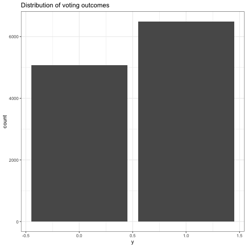

plot of chunk unnamed-chunk-4

Here’s the gender indicator.

data.frame(female) %>% 
  ggplot(aes(female)) +
  geom_bar() +
  ggtitle("Distribution of female indicator")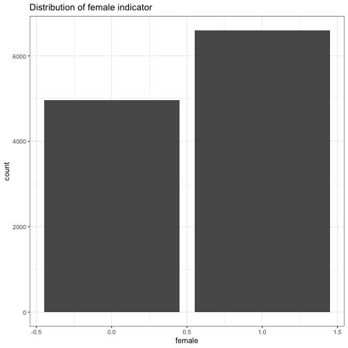

plot of chunk unnamed-chunk-5

Here’s the race indicator.

data.frame(black) %>% 
  ggplot(aes(black)) +
  geom_bar() +
  ggtitle("Distribution of black indicator")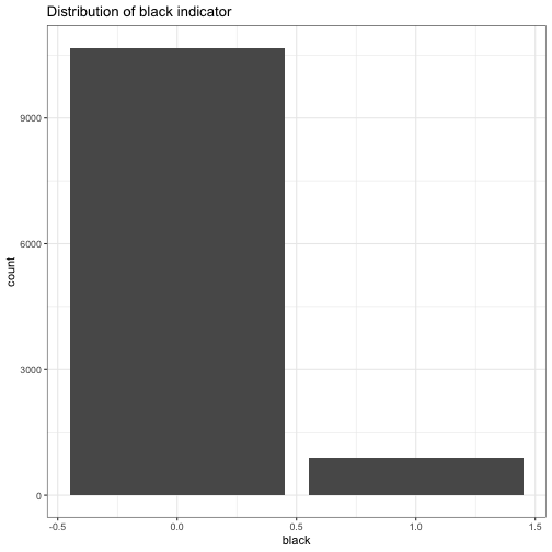

plot of chunk unnamed-chunk-6

Here’s the state variable. We have 51 state codes in the data, which includes Washington, DC.

data.frame(state) %>% 
  ggplot(aes(state)) +
  geom_bar() +
  ggtitle("Distribution of values within state")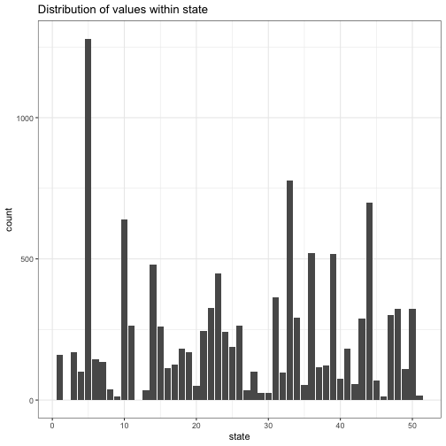

plot of chunk unnamed-chunk-7

On the other, there are no observations for states 2 or 12. We’ll drop them from the model.

state_recoded <- dplyr::dense_rank(state)
table(state_recoded)

## state_recoded
##    1    2    3    4    5    6    7    8    9   10   11   12   13   14   15   16 
##  159  168  101 1280  145  134   37   13  641  264   34  479  261  113  127  183 
##   17   18   19   20   21   22   23   24   25   26   27   28   29   30   31   32 
##  169   49  246  325  447  240  189  263   35  102   24   24  363   96  777  292 
##   33   34   35   36   37   38   39   40   41   42   43   44   45   46   47   48 
##   54  521  115  124  517   75  183   56  290  698   69   12  302  323  109  323 
##   49 
##   15

Building the model

Switching into greta, we’ll start by defining the data objects to use in our model.

n <- length(y)
n_states <- max(state_recoded)

y_greta <- as_data(y)
black_greta <- as_data(black)
female_greta <- as_data(female)
state_greta <- as_data(state_recoded)

Now, we’ll set up the model components. First, the random effects. To match the Stan code above, we’ll store all of these in an a vector. We specify the number of effects using the dim parameter below.

mu_a <- normal(0, 1)
sigma_a <- variable(lower = 0.0, upper = 100.0)
a <- normal(mu_a, sigma_a, dim = n_states)

We can use a similar approach to get the fixed effects in a single vector. We’ll have two effects.

b <- normal(0, 100, dim = 2)

We will define the distribution of the outcome variable, y, as a transformation of a linear combination of the inputs above.

y_hat <- b[1] * black_greta + b[2] * female_greta + a[state_recoded]
p <- ilogit(y_hat)
distribution(y_greta) <- binomial(n, p)

And finally, we assemble the components that we wish to sample in a model.

e88_model <- model(b, a, precision = "double")

Let’s check out our graph.

plot(e88_model)

## Error in `loadNamespace()`:
## ! there is no package called 'webshot'

Inference

Model in hand, we can begin sampling. Since we are sampling across multiple chains, we’ll use the “multisession” future strategy to do everything in parallel.

draws <- mcmc(e88_model, warmup = 1000, n_samples = 1000, chains = 4)

Time to diagnose. Did the sample chains for our fixed effects mix reasonably? For all of the following visualizations, we’ll rely on the bayesplot package.

bayesplot::mcmc_trace(draws, regex_pars = "b\\[[.[12]")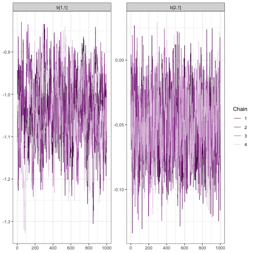

plot of chunk unnamed-chunk-16

And what about the random effects? We’ll investigate the first 5. Remember, we’ve recoded the previous state vector to remove the levels 2 and 12, which didn’t have any observations.

bayesplot::mcmc_trace(draws, regex_pars = "a\\[[1-5]\\,")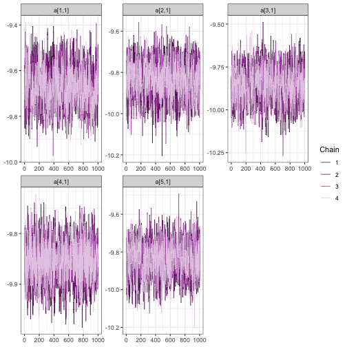

plot of chunk unnamed-chunk-17

Understanding our coefficients in their current form is a little hard, since they are on the logit scale. It would be nicer to work with probabilities. We can use calculate for this step.

To get every transformed version of our model parameters, we pass the draws object as the second argument. To get the name in an expected manner, we will assign the transformation to a local variable first.

prob <- ilogit(b)
as_probs <- calculate(prob, values = draws)

And now a plot.

mcmc_areas(as_probs)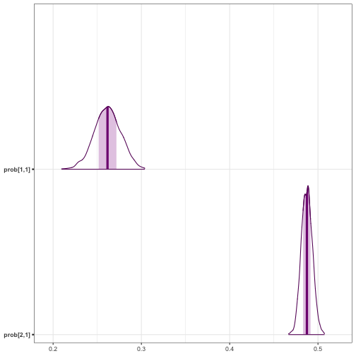

plot of chunk unnamed-chunk-19

And the summarized results.

summary(as_probs)

## 
## Iterations = 1:1000
## Thinning interval = 1 
## Number of chains = 4 
## Sample size per chain = 1000 
## 
## 1. Empirical mean and standard deviation for each variable,
##    plus standard error of the mean:
## 
##             Mean       SD  Naive SE Time-series SE
## prob[1,1] 0.2616 0.014947 2.363e-04      0.0008950
## prob[2,1] 0.4874 0.006173 9.761e-05      0.0001928
## 
## 2. Quantiles for each variable:
## 
##             2.5%    25%    50%    75%  97.5%
## prob[1,1] 0.2307 0.2516 0.2616 0.2717 0.2907
## prob[2,1] 0.4757 0.4831 0.4875 0.4916 0.4997

Wrapping up

We can finally go back to the question posed at this beginning of this example. During the 1988 election a black voter, from a randomly selected state, had a .25 to .27 probability of voting for Reagan, while women had .48 to .49 probability of voting for the Republican candidate.

Session information

sessionInfo()