greta#855 (tf-warmup-i547): effective samples from its warmup tuning

Effective samples per sampler iteration and per second of mcmc() with each version’s defaults on main and greta#855, on four of greta’s examples over twenty sessions. #855’s warmup tunes to larger step sizes, gives more effective samples per sampler iteration on three of the four models, and gives 2.8 to 7.9 times main’s effective samples per second.
Published

October 13, 2026

Setup
source(here::here("posts", "_helpers.R"))

post_path <- "posts/2026-10-13-tuning-efficiency-i547"
file_link <- file_linker(post_path)
section_link <- section_linker(post_path)
# the sections of benchmark.R, shown below by their labels
knitr::read_chunk(here(post_path, "benchmark.R"))

sessions <- read_sessions(post_path)
n_sessions <- length(sessions)

version_labels <- c(main = "main", `#855` = "#855")
versions <- display_versions(sessions[[1]]$versions, labels = version_labels)
version_levels <- names(versions)
colours <- version_colours(version_levels)
settings <- sessions[[1]]$results[[1]]$settings

# how the text names each version: main links to its commit, #855 to the PR
version_text <- c(
  main = paste0("[main](", commit_url(versions[["main"]]), ")"),
  `#855` = paste0("[#855](", pr_url(855), ")")
)
version_ref <- function(version) I(version_text[[version]])

# one row per session and version, holding that version's results
runs <- lapply(sessions, function(session_file) {
  tibble(
    session = session_file$session,
    version = factor(
      unname(version_labels[names(session_file$results)]),
      levels = version_levels
    ),
    results = unname(session_file$results)
  )
}) |>
  bind_rows()

model_levels <- names(runs$results[[1]]$mcmc)
# benchmark.R's section for each model
model_sections <- paste0("mcmc-", gsub("_", "-", model_levels))

# one row per run of mcmc(): its timed calls, the last call's draws, the
# sampler iterations each draw cost, and what warmup tuned hmc() to
mcmc_runs <- lapply(seq_len(nrow(runs)), function(i) {
  results <- runs$results[[i]]
  lapply(model_levels, function(model_name) {
    run <- results$mcmc[[model_name]]
    tibble(
      session = runs$session[i],
      version = runs$version[i],
      model = model_name,
      call_seconds = list(as.numeric(run$marks$time[[1]])),
      draws = list(run$draws),
      iterations_per_draw = results$sampler_iterations_per_draw,
      epsilon = run$epsilon,
      diag_sd = list(run$diag_sd)
    )
  }) |>
    bind_rows()
}) |>
  bind_rows() |>
  mutate(model = factor(model, levels = model_levels))

# small dots for the sessions over a large faint dot for their mean
gg_sessions <- function(data, means, measure, x_label) {
  ggplot(data, aes(x = {{ measure }}, y = version, colour = version)) +
    geom_point(data = means, size = 5, alpha = 0.25) +
    geom_point(
      position = position_jitter(width = 0, height = 0.2, seed = 2026),
      size = 1.2
    ) +
    scale_colour_manual(values = colours, guide = "none") +
    facet_wrap(vars(model), ncol = 2, scales = "free_x") +
    labs(x = x_label, y = NULL)
}
session_caption <- "Each small dot is one session's run. The large faint dot behind them is the mean of the sessions."

# what each "Run it yourself" block runs: setup, the iteration count, and every
# model
run_code <- run_it_yourself(
  post_path,
  "benchmark.R",
  c("setup", "sampler-iterations", model_sections),
  versions,
  paste0(
    "list(sampler_iterations_per_draw = sampler_iterations_per_draw, ",
    paste0(model_levels, " = mcmc_", model_levels, collapse = ", "),
    ")"
  )
)
The measures, and each version’s mean
# posterior caps a bulk ESS at S × log10(S) for S draws, which anticorrelated
# draws can reach, and warns each time. The warnings are counted here and
# reported under Convergence
ess_cap_warnings <- 0
summarise_counting_caps <- function(draws) {
  withCallingHandlers(
    posterior::summarise_draws(draws, "mean", "rhat", "ess_bulk", "ess_tail"),
    warning = function(w) {
      if (grepl("The ESS has been capped", conditionMessage(w), fixed = TRUE)) {
        ess_cap_warnings <<- ess_cap_warnings + 1
        invokeRestart("muffleWarning")
      }
    }
  )
}

# everything is from the run's last call, whose draws were kept
efficiency <- mcmc_runs |>
  mutate(
    posterior = lapply(draws, summarise_counting_caps),
    n_draws = vapply(draws, posterior::ndraws, numeric(1)),
    seconds = vapply(
      call_seconds,
      \(times) times[[settings$mcmc_calls]],
      numeric(1)
    ),
    smallest_ess_bulk = vapply(posterior, \(summary) min(summary$ess_bulk), numeric(1)),
    smallest_ess_tail = vapply(posterior, \(summary) min(summary$ess_tail), numeric(1)),
    largest_rhat = vapply(posterior, \(summary) max(summary$rhat), numeric(1)),
    smallest_ess_capped = smallest_ess_bulk >=
      n_draws * log10(n_draws) * (1 - 1e-9),
    sampler_iterations = n_draws * iterations_per_draw,
    ess_per_iteration = smallest_ess_bulk / sampler_iterations,
    ess_per_second = smallest_ess_bulk / seconds
  ) |>
  select(-call_seconds, -draws, -diag_sd, -posterior)

# each version's mean over the sessions, for each model
efficiency_means <- efficiency |>
  group_by(model, version) |>
  summarise(
    across(c(epsilon, ess_per_iteration, ess_per_second), mean),
    .groups = "drop"
  )

# #855's mean over main's, for each model
pr_over_main <- efficiency_means |>
  pivot_longer(
    c(epsilon, ess_per_iteration, ess_per_second),
    names_to = "measure"
  ) |>
  pivot_wider(names_from = version, values_from = value) |>
  mutate(ratio = `#855` / main)
ratio_of <- function(measure_name, model_name) {
  pr_over_main$ratio[
    pr_over_main$measure == measure_name & pr_over_main$model == model_name
  ]
}

# "#855 gives 1.4 times main's", for one measure and model
compare_on <- function(measure_name, model_name) {
  compare_rates(
    ratio_of(measure_name, model_name),
    version_text[["#855"]],
    version_text[["main"]]
  )
}

greta#855 runs hmc()’s warmup inside TensorFlow, and its warmup tunes the step size to different values from main’s. This post runs main and #855 with each version’s defaults on four of greta’s examples, in 20 sessions, to see whether that changes how many effective samples mcmc() gives. Taking the smallest bulk ESS of each run, and each version’s mean over the sessions, per sampler iteration (which leaves out how fast the code runs) and per second:

The versions.

  • main: greta-dev/greta@73015623. Each draw costs thin + 1 sampler iterations, two at the default thin = 1, and each warmup step runs the same way, so its defaults of warmup = 1000 and n_samples = 1000 run 2000 iterations in each phase. It tunes epsilon and diag_sd in R between bursts of three warmup steps, and draws hmc()’s number of leapfrog steps once per burst.
  • #855: greta-dev/greta@f6df0064. Each draw and each warmup step is one sampler iteration, and its defaults of warmup = 2000 and n_samples = 2000 run the same 2000 iterations in each phase as main’s. It tunes inside TensorFlow every three iterations, on the same schedule as main: epsilon by dual averaging (Hoffman and Gelman 2014) over the first 10% and last 60% of warmup, diag_sd between 10% and 40%. It draws the number of leapfrog steps afresh every iteration.

The models, four of greta’s examples. Normal and log-normal distributions are written with their mean and standard deviation, as greta’s normal() and lognormal() take them; \(\text{Cauchy}^{+}\) is a Cauchy truncated to positive values.

Each department’s rating in attitude regressed on its number of complaints.

\[ \begin{aligned} \text{rating}_i &\sim \text{Normal}(\mu_i, \sigma), \quad i = 1, \dots, 30 \\ \mu_i &= \alpha + \beta \, \text{complaints}_i \\ \alpha, \beta &\sim \text{Normal}(0, 10) \\ \sigma &\sim \text{Cauchy}^{+}(0, 3) \end{aligned} \]

benchmark.R: mcmc-linear
# greta's linear example: the rating of each department in `attitude`
# regressed on its complaints
mcmc_linear <- local({
  int <- normal(0, 10)
  coef <- normal(0, 10)
  sd <- cauchy(0, 3, truncation = c(0, Inf))
  mu <- int + coef * attitude$complaints
  distribution(attitude$rating) <- normal(mu, sd)
  m <- model(int, coef, sd)
  time_mcmc(m)
})

The same rating on all six of attitude’s other columns, \(X\), through a matrix multiply.

\[ \begin{aligned} \text{rating}_i &\sim \text{Normal}(\mu_i, \sigma), \quad i = 1, \dots, 30 \\ \mu_i &= \alpha + \sum_{j = 1}^{6} X_{ij} \, \beta_j \\ \alpha, \beta_j &\sim \text{Normal}(0, 10) \\ \sigma &\sim \text{Cauchy}^{+}(0, 3) \end{aligned} \]

benchmark.R: mcmc-multiple-linear
# the same rating on all six of `attitude`'s other columns
mcmc_multiple_linear <- local({
  design <- as.matrix(attitude[, 2:7])
  int <- normal(0, 10)
  coefs <- normal(0, 10, dim = ncol(design))
  sd <- cauchy(0, 3, truncation = c(0, Inf))
  mu <- int + design %*% coefs
  distribution(attitude$rating) <- normal(mu, sd)
  m <- model(int, coefs, sd)
  time_mcmc(m)
})

Sepal length on sepal width in iris, with an offset for each species, \(s[i]\) being flower \(i\)’s. Setosa’s offset is zero and the other two share a scale, \(\tau\).

\[ \begin{aligned} \text{Sepal.Length}_i &\sim \text{Normal}(\mu_i, \sigma), \quad i = 1, \dots, 150 \\ \mu_i &= \alpha + \beta \, \text{Sepal.Width}_i + \gamma_{s[i]} \\ \gamma_1 &= 0, \qquad \gamma_2, \gamma_3 \sim \text{Normal}(0, \tau) \\ \tau &\sim \text{LogNormal}(0, 1) \\ \alpha, \beta &\sim \text{Normal}(0, 10) \\ \sigma &\sim \text{Cauchy}^{+}(0, 3) \end{aligned} \]

benchmark.R: mcmc-hierarchical-linear
# sepal length on sepal width in `iris`, with an offset for each species
mcmc_hierarchical_linear <- local({
  int <- normal(0, 10)
  coef <- normal(0, 10)
  sd <- cauchy(0, 3, truncation = c(0, Inf))
  species_sd <- lognormal(0, 1)
  species_offset <- normal(0, species_sd, dim = 2)
  species_effect <- rbind(0, species_offset)
  species_id <- as.numeric(iris$Species)
  mu <- int + coef * iris$Sepal.Width + species_effect[species_id]
  distribution(iris$Sepal.Length) <- normal(mu, sd)
  m <- model(int, coef, sd, species_sd, species_offset)
  time_mcmc(m)
})

The effect of coaching in eight schools, \(y_j\), each measured with a known standard error, \(\sigma_j\). The scale of the school effects, \(\sigma_\eta\), is itself a parameter, which makes the posterior a funnel.

\[ \begin{aligned} y_j &\sim \text{Normal}(\theta_j, \sigma_j), \quad j = 1, \dots, 8 \\ \theta_j &= \mu + \xi \, \eta_j \\ \eta_j &\sim \text{Normal}(0, \sigma_\eta) \\ \sigma_\eta &\sim \text{InverseGamma}(1, 1) \\ \mu &\sim \text{Normal}(0, 100) \\ \xi &\sim \text{Normal}(0, 5) \end{aligned} \]

benchmark.R: mcmc-eight-schools
# the effect of coaching in eight schools, each measured with a known
# standard error
mcmc_eight_schools <- local({
  y <- c(28, 8, -3, 7, -1, 1, 18, 12)
  sigma_y <- c(15, 10, 16, 11, 9, 11, 10, 18)
  sigma_eta <- inverse_gamma(1, 1)
  eta <- normal(0, sigma_eta, dim = 8)
  mu_theta <- normal(0, 100)
  xi <- normal(0, 5)
  theta <- mu_theta + xi * eta
  distribution(y) <- normal(theta, sigma_y)
  m <- model(sigma_eta, eta, mu_theta, xi)
  time_mcmc(m)
})

What was run. In each session, each version ran mcmc() with 4 chains, verbose = FALSE, the default sampler, hmc(), and its own default warmup and n_samples on each model, calling it 2 times on the model, the first call tracing it. Everything here is from the last call: its runtime, its draws, and the epsilon and diag_sd warmup tuned, read from the result (time_mcmc(), in the setup section).

What was measured. The bulk effective sample size (ESS) (Vehtari et al. 2021) of each run’s worst-mixing parameter, as Hoffman and Gelman (2014) report it:

  • per sampler iteration of the sampling phase: the draws, times the sampler iterations each draw costs, which the sampler-iterations section counts with a random walk. Both versions draw the number of leapfrog steps uniformly from 5 to 10, so this is in proportion to ESS per gradient evaluation. It is what the tuning gives, apart from how fast the code runs.
  • per second of the call, warmup included: the time-normalised ESS of Girolami and Calderhead (2011), which is what a user gets.

The sessions. run.R installed each version as its run-versions section says, and ran benchmark.R for each in a fresh R session of its own, in 20 sessions, the order rotating so that each version ran first equally often (its run-sessions section). Each session gives each version one seed, session_seed. Every version ran on TensorFlow 2.21.0, TensorFlow Probability 0.25.0 and reticulate 1.47.0, on Darwin 25.5.0 arm64 with 8 cores.

The scripts in full.

run.R
# Runs benchmark.R against main and greta#855, in a fresh R session per
# version, in twenty sessions:
#
#   Rscript --quiet --vanilla posts/2026-10-13-tuning-efficiency-i547/run.R
#
# Each session writes results/session-<n>.rds, and sessions already there are
# skipped, so a rerun after a crash carries on. Each `# ---- label ----` line
# starts a section that index.qmd shows by that label. Keep the machine idle
# while it runs, and on mains power, with the lid open: a session that
# overlaps other work, or a sleep, is not a measurement.

# ---- run-versions ----
# Pin every version to a commit: branches move, and the post links each one.
# The version the post is about goes last, which is where the page's colours
# expect it.
versions <- c(
  main = "greta-dev/greta@730156234aaa390f5091cdcecc018af891d3e28c",
  `#855` = "greta-dev/greta@f6df0064137f9cec8d14e93128c8c6feef322770"
)
# a multiple of the number of versions, so each takes each place in the order
# equally often. Each session gives each version one seed, and the step size
# warmup tunes to varies from seed to seed, so this takes more sessions than a
# timing alone would
n_sessions <- 20
post_dir <- here::here("posts", "2026-10-13-tuning-efficiency-i547")

# ---- run-sessions ----
dir.create(file.path(post_dir, "results"), showWarnings = FALSE)

for (session in seq_len(n_sessions)) {
  session_file <- file.path(
    post_dir,
    "results",
    sprintf("session-%d.rds", session)
  )
  if (file.exists(session_file)) {
    next
  }

  # The version that runs first in a session tends to be the slower, so the
  # order rotates: each session starts one place further along. A random order
  # can put one version first in four sessions of five, which then reads as a
  # difference between the versions.
  start <- (session - 1) %% length(versions)
  order <- names(versions)[
    (seq_along(versions) + start - 1) %%
      length(versions) +
      1
  ]

  # cross::run_versions() installs each version into a library of its own and
  # evaluates the expression in a fresh R session against it. That session
  # cannot see this one's variables, so the script's path and the session
  # number reach it as environment variables: args_callr is passed on to
  # callr::r(), whose `env` sets variables for the child process (see ?callr::r
  # and ?callr::rcmd_safe_env, whose defaults are kept).
  measured <- cross::run_versions(
    source(Sys.getenv("GRETA_BENCH_SCRIPT"), local = TRUE)$value,
    pkgs = unname(versions[order]),
    args_callr = list(
      env = c(
        callr::rcmd_safe_env(),
        GRETA_BENCH_SCRIPT = file.path(post_dir, "benchmark.R"),
        GRETA_BENCH_SESSION = session
      )
    )
  )

  saveRDS(
    list(
      session = session,
      versions = versions,
      order = order,
      results = setNames(measured$result, order)
    ),
    session_file,
    compress = "xz"
  )
}
benchmark.R
# What each version of greta runs, in a fresh R session of its own: run.R
# sources it once per version per session, and keeps the list it ends with.
#
# Each `# ---- label ----` line starts a section. The post shows each one by
# its label, links to it under the figure it fed, and builds that figure's
# "Run it yourself" block from `setup` and the figure's own section. So keep
# every timed section self-contained: it builds its own model and reads only
# `setup`'s settings, so that `setup` plus that one section run on their own.
#
# Run it alone to try it against whichever greta is installed:
#
#   Rscript --quiet --vanilla posts/2026-10-13-tuning-efficiency-i547/benchmark.R

# ---- setup ----
library(greta)
library(bench)
session <- as.integer(Sys.getenv("GRETA_BENCH_SESSION", "1"))
# the date the post was started, as a seed
session_seed <- 2026 - 10 - 13 + session
# mcmc() runs with each version's own default warmup and n_samples.
# mcmc_calls counts timed calls on one model, the first of which traces
settings <- list(
  chains = 4,
  mcmc_calls = 2
)

# Times mcmc() on a model, and keeps the last call's draws and the epsilon and
# diag_sd that warmup tuned hmc() to
time_mcmc <- function(m) {
  set.seed(session_seed)
  marks <- mark(
    draws <- mcmc(m, chains = settings$chains, verbose = FALSE),
    iterations = settings$mcmc_calls,
    check = FALSE,
    memory = FALSE,
    filter_gc = FALSE
  )
  tuned <- attr(draws, "model_info")$samplers[[1]]$parameters
  list(
    marks = marks,
    draws = posterior::as_draws_array(draws),
    epsilon = tuned$epsilon,
    diag_sd = as.numeric(tuned$diag_sd)
  )
}

# ---- sampler-iterations ----
# A random walk on a target far wider than its steps accepts every proposal, so
# the variance between kept draws over one step's variance counts the sampler
# iterations between them. It is also the session's first mcmc() call, so
# TensorFlow's start-up costs fall here rather than on the first model
sampler_iterations_per_draw <- local({
  step_sd <- 0.1
  x <- normal(0, 1e6)
  m <- model(x)
  walk <- mcmc(
    m,
    sampler = rwmh(epsilon = step_sd, diag_sd = 1),
    warmup = 0,
    n_samples = 4000,
    chains = 1,
    initial_values = initials(x = 0),
    verbose = FALSE
  )
  round(var(diff(as.vector(walk[[1]]))) / step_sd^2)
})

# ---- mcmc-linear ----
# greta's linear example: the rating of each department in `attitude`
# regressed on its complaints
mcmc_linear <- local({
  int <- normal(0, 10)
  coef <- normal(0, 10)
  sd <- cauchy(0, 3, truncation = c(0, Inf))
  mu <- int + coef * attitude$complaints
  distribution(attitude$rating) <- normal(mu, sd)
  m <- model(int, coef, sd)
  time_mcmc(m)
})

# ---- mcmc-multiple-linear ----
# the same rating on all six of `attitude`'s other columns
mcmc_multiple_linear <- local({
  design <- as.matrix(attitude[, 2:7])
  int <- normal(0, 10)
  coefs <- normal(0, 10, dim = ncol(design))
  sd <- cauchy(0, 3, truncation = c(0, Inf))
  mu <- int + design %*% coefs
  distribution(attitude$rating) <- normal(mu, sd)
  m <- model(int, coefs, sd)
  time_mcmc(m)
})

# ---- mcmc-hierarchical-linear ----
# sepal length on sepal width in `iris`, with an offset for each species
mcmc_hierarchical_linear <- local({
  int <- normal(0, 10)
  coef <- normal(0, 10)
  sd <- cauchy(0, 3, truncation = c(0, Inf))
  species_sd <- lognormal(0, 1)
  species_offset <- normal(0, species_sd, dim = 2)
  species_effect <- rbind(0, species_offset)
  species_id <- as.numeric(iris$Species)
  mu <- int + coef * iris$Sepal.Width + species_effect[species_id]
  distribution(iris$Sepal.Length) <- normal(mu, sd)
  m <- model(int, coef, sd, species_sd, species_offset)
  time_mcmc(m)
})

# ---- mcmc-eight-schools ----
# the effect of coaching in eight schools, each measured with a known
# standard error
mcmc_eight_schools <- local({
  y <- c(28, 8, -3, 7, -1, 1, 18, 12)
  sigma_y <- c(15, 10, 16, 11, 9, 11, 10, 18)
  sigma_eta <- inverse_gamma(1, 1)
  eta <- normal(0, sigma_eta, dim = 8)
  mu_theta <- normal(0, 100)
  xi <- normal(0, 5)
  theta <- mu_theta + xi * eta
  distribution(y) <- normal(theta, sigma_y)
  m <- model(sigma_eta, eta, mu_theta, xi)
  time_mcmc(m)
})

# ---- provenance ----
session_info <- sessioninfo::session_info()
# greta_sitrep() reports through messages, so capture those
greta_sitrep_report <- utils::capture.output(greta_sitrep(), type = "message")
tf <- tensorflow::tf
tfp <- reticulate::import("tensorflow_probability")
greta_sha <- packageDescription("greta")$RemoteSha
provenance <- data.frame(
  greta_version = as.character(packageVersion("greta")),
  greta_sha = if (is.null(greta_sha)) NA_character_ else greta_sha,
  r_version = paste(R.version$major, R.version$minor, sep = "."),
  tensorflow_version = tf$version$VERSION,
  tfp_version = tfp$`__version__`,
  reticulate_version = as.character(packageVersion("reticulate")),
  machine = paste(
    Sys.info()[c("sysname", "release", "machine")],
    collapse = " "
  ),
  cores = parallel::detectCores()
)

# ---- results ----
# the value source() returns to run.R: every bench_mark object as mark() made
# it, so summary() and autoplot() work on it, with each run's draws and tuned
# values beside it
list(
  session_seed = session_seed,
  settings = settings,
  provenance = provenance,
  session_info = session_info,
  greta_sitrep_report = greta_sitrep_report,
  sampler_iterations_per_draw = sampler_iterations_per_draw,
  mcmc = list(
    linear = mcmc_linear,
    multiple_linear = mcmc_multiple_linear,
    hierarchical_linear = mcmc_hierarchical_linear,
    eight_schools = mcmc_eight_schools
  )
)
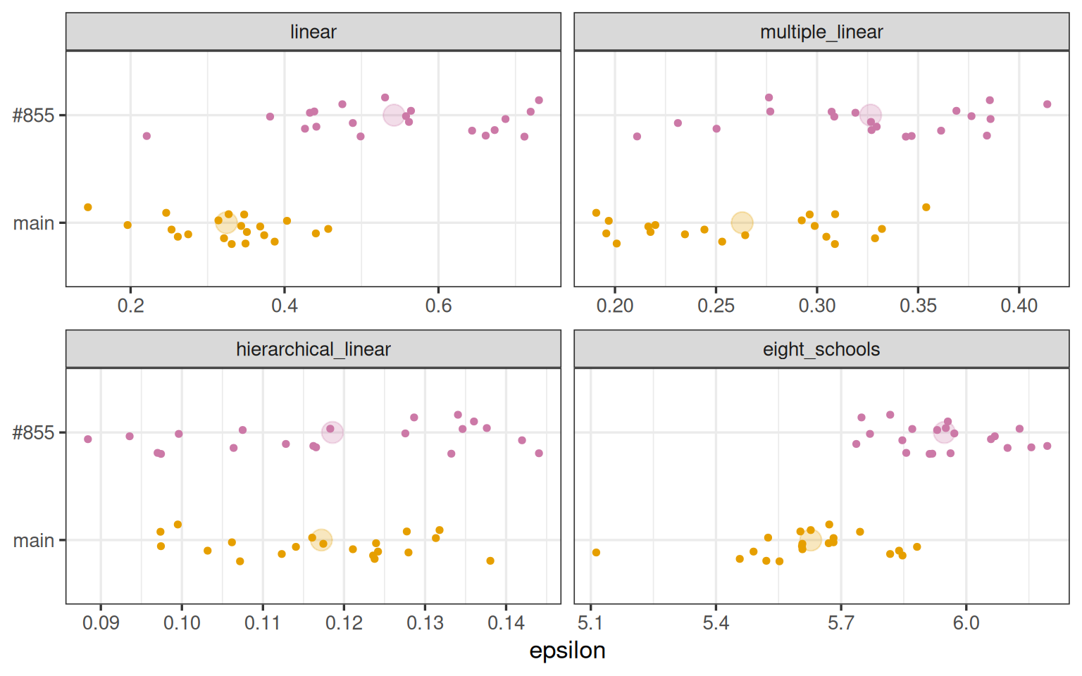
Step size warmup tunes to

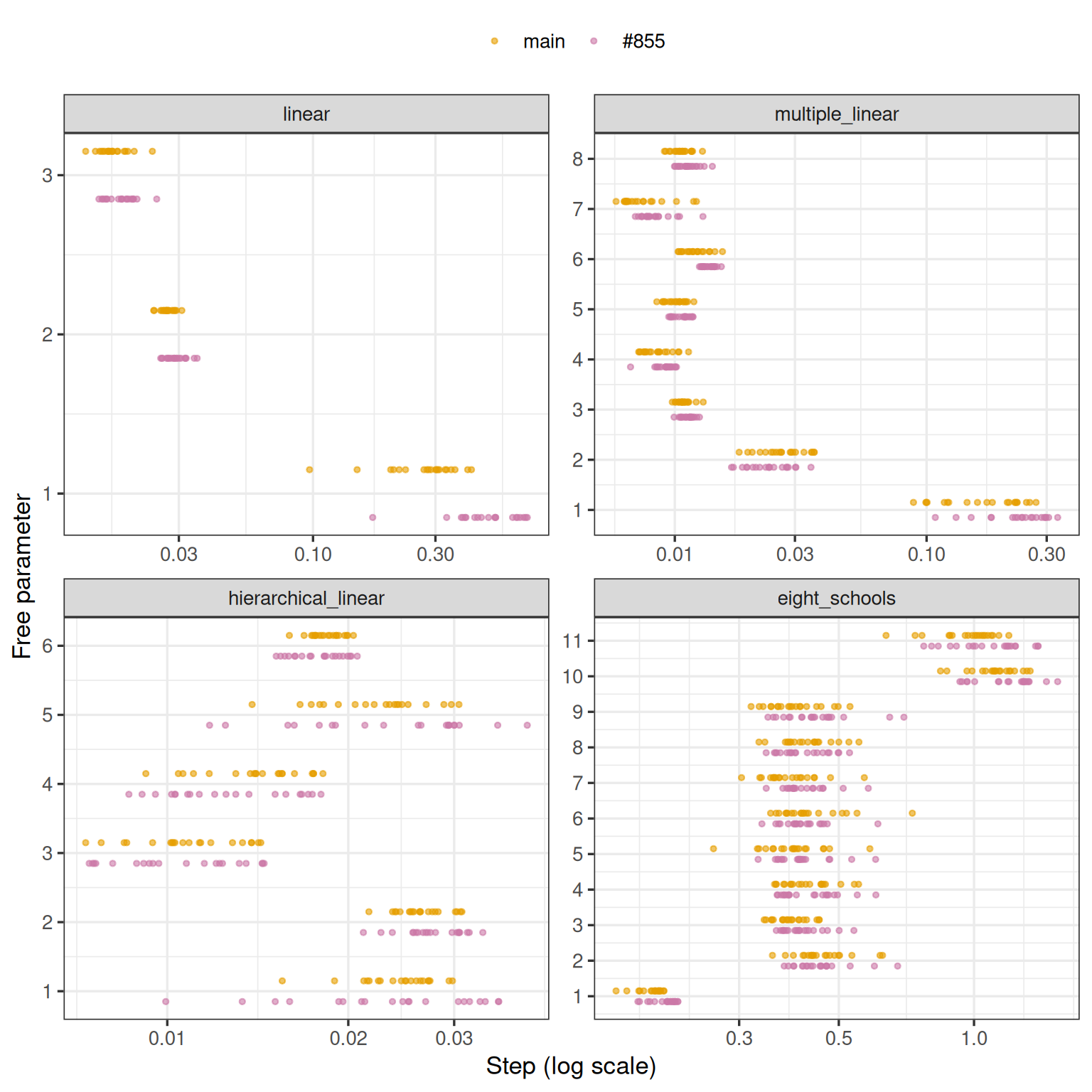
epsilon, the step size hmc() takes after warmup, in each run. Each parameter’s step is epsilon times its diag_sd over the sum of diag_sd, so epsilon is the sum of the parameters’ steps.

Code
gg_sessions(efficiency, efficiency_means, epsilon, "epsilon")

Each small dot is one session’s run. The large faint dot behind them is the mean of the sessions.

Tuned by benchmark.R’s setup, mcmc-linear, mcmc-multiple-linear, mcmc-hierarchical-linear and mcmc-eight-schools sections.

Run it yourself
# install.packages(c("pak", "bench"))
# pak::pak("DavisVaughan/cross")
results <- cross::run_versions(
  {
    # ---- setup ----
    library(greta)
    library(bench)
    session <- as.integer(Sys.getenv("GRETA_BENCH_SESSION", "1"))
    # the date the post was started, as a seed
    session_seed <- 2026 - 10 - 13 + session
    # mcmc() runs with each version's own default warmup and n_samples.
    # mcmc_calls counts timed calls on one model, the first of which traces
    settings <- list(
      chains = 4,
      mcmc_calls = 2
    )

    # Times mcmc() on a model, and keeps the last call's draws and the epsilon and
    # diag_sd that warmup tuned hmc() to
    time_mcmc <- function(m) {
      set.seed(session_seed)
      marks <- mark(
        draws <- mcmc(m, chains = settings$chains, verbose = FALSE),
        iterations = settings$mcmc_calls,
        check = FALSE,
        memory = FALSE,
        filter_gc = FALSE
      )
      tuned <- attr(draws, "model_info")$samplers[[1]]$parameters
      list(
        marks = marks,
        draws = posterior::as_draws_array(draws),
        epsilon = tuned$epsilon,
        diag_sd = as.numeric(tuned$diag_sd)
      )
    }
    # ---- sampler-iterations ----
    # A random walk on a target far wider than its steps accepts every proposal, so
    # the variance between kept draws over one step's variance counts the sampler
    # iterations between them. It is also the session's first mcmc() call, so
    # TensorFlow's start-up costs fall here rather than on the first model
    sampler_iterations_per_draw <- local({
      step_sd <- 0.1
      x <- normal(0, 1e6)
      m <- model(x)
      walk <- mcmc(
        m,
        sampler = rwmh(epsilon = step_sd, diag_sd = 1),
        warmup = 0,
        n_samples = 4000,
        chains = 1,
        initial_values = initials(x = 0),
        verbose = FALSE
      )
      round(var(diff(as.vector(walk[[1]]))) / step_sd^2)
    })
    # ---- mcmc-linear ----
    # greta's linear example: the rating of each department in `attitude`
    # regressed on its complaints
    mcmc_linear <- local({
      int <- normal(0, 10)
      coef <- normal(0, 10)
      sd <- cauchy(0, 3, truncation = c(0, Inf))
      mu <- int + coef * attitude$complaints
      distribution(attitude$rating) <- normal(mu, sd)
      m <- model(int, coef, sd)
      time_mcmc(m)
    })
    # ---- mcmc-multiple-linear ----
    # the same rating on all six of `attitude`'s other columns
    mcmc_multiple_linear <- local({
      design <- as.matrix(attitude[, 2:7])
      int <- normal(0, 10)
      coefs <- normal(0, 10, dim = ncol(design))
      sd <- cauchy(0, 3, truncation = c(0, Inf))
      mu <- int + design %*% coefs
      distribution(attitude$rating) <- normal(mu, sd)
      m <- model(int, coefs, sd)
      time_mcmc(m)
    })
    # ---- mcmc-hierarchical-linear ----
    # sepal length on sepal width in `iris`, with an offset for each species
    mcmc_hierarchical_linear <- local({
      int <- normal(0, 10)
      coef <- normal(0, 10)
      sd <- cauchy(0, 3, truncation = c(0, Inf))
      species_sd <- lognormal(0, 1)
      species_offset <- normal(0, species_sd, dim = 2)
      species_effect <- rbind(0, species_offset)
      species_id <- as.numeric(iris$Species)
      mu <- int + coef * iris$Sepal.Width + species_effect[species_id]
      distribution(iris$Sepal.Length) <- normal(mu, sd)
      m <- model(int, coef, sd, species_sd, species_offset)
      time_mcmc(m)
    })
    # ---- mcmc-eight-schools ----
    # the effect of coaching in eight schools, each measured with a known
    # standard error
    mcmc_eight_schools <- local({
      y <- c(28, 8, -3, 7, -1, 1, 18, 12)
      sigma_y <- c(15, 10, 16, 11, 9, 11, 10, 18)
      sigma_eta <- inverse_gamma(1, 1)
      eta <- normal(0, sigma_eta, dim = 8)
      mu_theta <- normal(0, 100)
      xi <- normal(0, 5)
      theta <- mu_theta + xi * eta
      distribution(y) <- normal(theta, sigma_y)
      m <- model(sigma_eta, eta, mu_theta, xi)
      time_mcmc(m)
    })
    # the timings to bring back
    list(sampler_iterations_per_draw = sampler_iterations_per_draw, linear = mcmc_linear, multiple_linear = mcmc_multiple_linear, hierarchical_linear = mcmc_hierarchical_linear, eight_schools = mcmc_eight_schools)
  },
  pkgs = c(
    "greta-dev/greta@730156234aaa390f5091cdcecc018af891d3e28c",
    "greta-dev/greta@f6df0064137f9cec8d14e93128c8c6feef322770"
  )
)
Code
# "#855's is 1.2 to 1.5 times main's" over the models, naming the version
# with the larger mean epsilon
epsilon_ratios <- pr_over_main$ratio[pr_over_main$measure == "epsilon"]
pr_epsilon <- paste0(version_text[["#855"]], "'s")
main_epsilon <- paste0(version_text[["main"]], "'s")
larger_epsilon <- if (all(epsilon_ratios >= 1)) {
  paste(pr_epsilon, "is", format_range(epsilon_ratios), "times", main_epsilon)
} else if (all(epsilon_ratios <= 1)) {
  paste(main_epsilon, "is", format_range(1 / epsilon_ratios), "times", pr_epsilon)
} else {
  paste0(
    "it varies: ",
    pr_epsilon,
    " is up to ",
    format_number(max(epsilon_ratios)),
    " times ",
    main_epsilon,
    ", and ",
    main_epsilon,
    " up to ",
    format_number(max(1 / epsilon_ratios)),
    " times ",
    pr_epsilon
  )
}

Over the four models, #855’s is 1.01 to 1.67 times main’s.

Figure: each parameter’s step
Code
steps <- mcmc_runs |>
  mutate(
    step = Map(
      \(epsilon, diag_sd) epsilon * diag_sd / sum(diag_sd),
      epsilon,
      diag_sd
    )
  ) |>
  select(session, version, model, step) |>
  mutate(parameter = lapply(step, seq_along)) |>
  unnest(c(step, parameter)) |>
  # each version's dots a little above or below their parameter's line
  mutate(row = parameter + ifelse(version == "main", 0.15, -0.15))

ggplot(steps, aes(x = step, y = row, colour = version)) +
  geom_point(size = 1, alpha = 0.6) +
  scale_x_log10() +
  scale_y_continuous(breaks = \(limits) seq(1, floor(limits[2]))) +
  scale_colour_manual(values = colours) +
  facet_wrap(vars(model), ncol = 2, scales = "free") +
  labs(x = "Step (log scale)", y = "Free parameter", colour = NULL) +
  theme(legend.position = "top")

Each dot is one session’s run. The free parameters are numbered in the order greta keeps them, on the scale hmc() samples them on.

Effective samples per sampler iteration

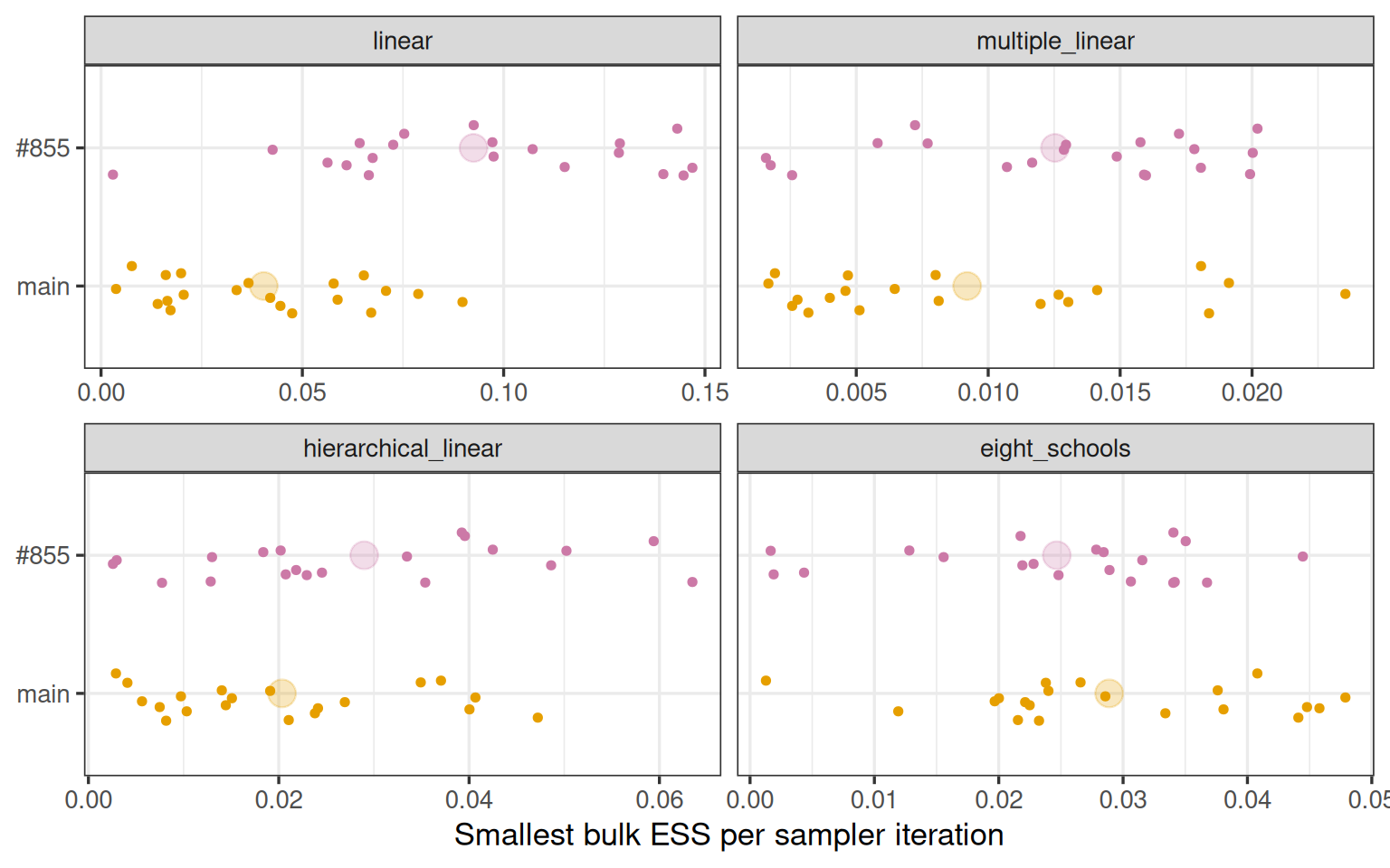
The smallest bulk ESS of each run over the sampler iterations of its sampling phase: how well the tuned sampler mixes, apart from how fast the code runs.

Code
gg_sessions(
  efficiency,
  efficiency_means,
  ess_per_iteration,
  "Smallest bulk ESS per sampler iteration"
)

Each small dot is one session’s run. The large faint dot behind them is the mean of the sessions.

Run by benchmark.R’s setup, sampler-iterations, mcmc-linear, mcmc-multiple-linear, mcmc-hierarchical-linear and mcmc-eight-schools sections.

Run it yourself
# install.packages(c("pak", "bench"))
# pak::pak("DavisVaughan/cross")
results <- cross::run_versions(
  {
    # ---- setup ----
    library(greta)
    library(bench)
    session <- as.integer(Sys.getenv("GRETA_BENCH_SESSION", "1"))
    # the date the post was started, as a seed
    session_seed <- 2026 - 10 - 13 + session
    # mcmc() runs with each version's own default warmup and n_samples.
    # mcmc_calls counts timed calls on one model, the first of which traces
    settings <- list(
      chains = 4,
      mcmc_calls = 2
    )

    # Times mcmc() on a model, and keeps the last call's draws and the epsilon and
    # diag_sd that warmup tuned hmc() to
    time_mcmc <- function(m) {
      set.seed(session_seed)
      marks <- mark(
        draws <- mcmc(m, chains = settings$chains, verbose = FALSE),
        iterations = settings$mcmc_calls,
        check = FALSE,
        memory = FALSE,
        filter_gc = FALSE
      )
      tuned <- attr(draws, "model_info")$samplers[[1]]$parameters
      list(
        marks = marks,
        draws = posterior::as_draws_array(draws),
        epsilon = tuned$epsilon,
        diag_sd = as.numeric(tuned$diag_sd)
      )
    }
    # ---- sampler-iterations ----
    # A random walk on a target far wider than its steps accepts every proposal, so
    # the variance between kept draws over one step's variance counts the sampler
    # iterations between them. It is also the session's first mcmc() call, so
    # TensorFlow's start-up costs fall here rather than on the first model
    sampler_iterations_per_draw <- local({
      step_sd <- 0.1
      x <- normal(0, 1e6)
      m <- model(x)
      walk <- mcmc(
        m,
        sampler = rwmh(epsilon = step_sd, diag_sd = 1),
        warmup = 0,
        n_samples = 4000,
        chains = 1,
        initial_values = initials(x = 0),
        verbose = FALSE
      )
      round(var(diff(as.vector(walk[[1]]))) / step_sd^2)
    })
    # ---- mcmc-linear ----
    # greta's linear example: the rating of each department in `attitude`
    # regressed on its complaints
    mcmc_linear <- local({
      int <- normal(0, 10)
      coef <- normal(0, 10)
      sd <- cauchy(0, 3, truncation = c(0, Inf))
      mu <- int + coef * attitude$complaints
      distribution(attitude$rating) <- normal(mu, sd)
      m <- model(int, coef, sd)
      time_mcmc(m)
    })
    # ---- mcmc-multiple-linear ----
    # the same rating on all six of `attitude`'s other columns
    mcmc_multiple_linear <- local({
      design <- as.matrix(attitude[, 2:7])
      int <- normal(0, 10)
      coefs <- normal(0, 10, dim = ncol(design))
      sd <- cauchy(0, 3, truncation = c(0, Inf))
      mu <- int + design %*% coefs
      distribution(attitude$rating) <- normal(mu, sd)
      m <- model(int, coefs, sd)
      time_mcmc(m)
    })
    # ---- mcmc-hierarchical-linear ----
    # sepal length on sepal width in `iris`, with an offset for each species
    mcmc_hierarchical_linear <- local({
      int <- normal(0, 10)
      coef <- normal(0, 10)
      sd <- cauchy(0, 3, truncation = c(0, Inf))
      species_sd <- lognormal(0, 1)
      species_offset <- normal(0, species_sd, dim = 2)
      species_effect <- rbind(0, species_offset)
      species_id <- as.numeric(iris$Species)
      mu <- int + coef * iris$Sepal.Width + species_effect[species_id]
      distribution(iris$Sepal.Length) <- normal(mu, sd)
      m <- model(int, coef, sd, species_sd, species_offset)
      time_mcmc(m)
    })
    # ---- mcmc-eight-schools ----
    # the effect of coaching in eight schools, each measured with a known
    # standard error
    mcmc_eight_schools <- local({
      y <- c(28, 8, -3, 7, -1, 1, 18, 12)
      sigma_y <- c(15, 10, 16, 11, 9, 11, 10, 18)
      sigma_eta <- inverse_gamma(1, 1)
      eta <- normal(0, sigma_eta, dim = 8)
      mu_theta <- normal(0, 100)
      xi <- normal(0, 5)
      theta <- mu_theta + xi * eta
      distribution(y) <- normal(theta, sigma_y)
      m <- model(sigma_eta, eta, mu_theta, xi)
      time_mcmc(m)
    })
    # the timings to bring back
    list(sampler_iterations_per_draw = sampler_iterations_per_draw, linear = mcmc_linear, multiple_linear = mcmc_multiple_linear, hierarchical_linear = mcmc_hierarchical_linear, eight_schools = mcmc_eight_schools)
  },
  pkgs = c(
    "greta-dev/greta@730156234aaa390f5091cdcecc018af891d3e28c",
    "greta-dev/greta@f6df0064137f9cec8d14e93128c8c6feef322770"
  )
)

On linear, #855 gives 2.29 times main’s; on multiple_linear, #855 gives 1.36 times main’s; on hierarchical_linear, #855 gives 1.42 times main’s; and on eight_schools, main gives 1.17 times #855’s.

Effective samples per second

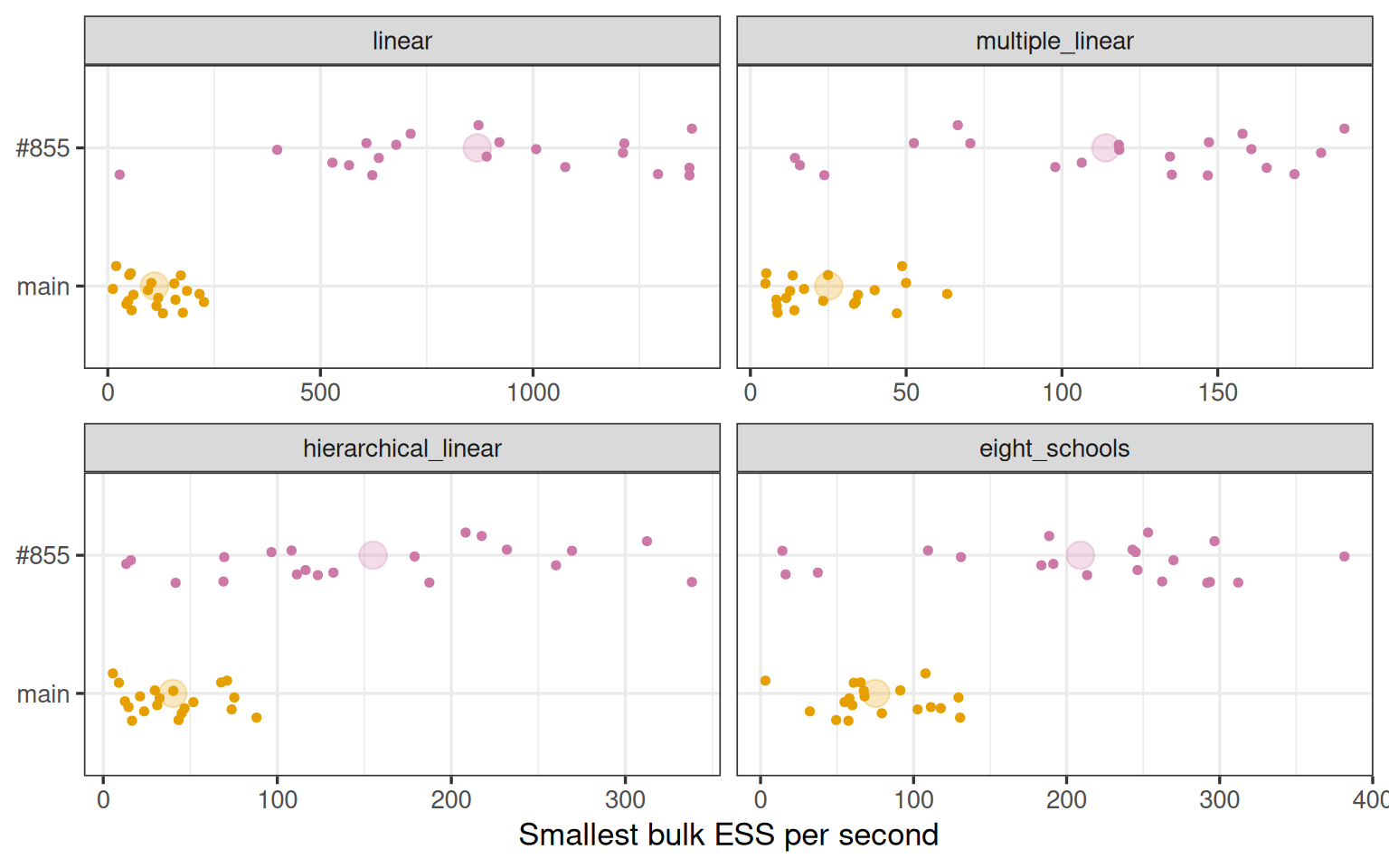
The smallest bulk ESS of each run per second of its last call, warmup included.

Code
gg_sessions(
  efficiency,
  efficiency_means,
  ess_per_second,
  "Smallest bulk ESS per second"
)

Each small dot is one session’s run. The large faint dot behind them is the mean of the sessions.

Timed by benchmark.R’s setup, mcmc-linear, mcmc-multiple-linear, mcmc-hierarchical-linear and mcmc-eight-schools sections.

Run it yourself
# install.packages(c("pak", "bench"))
# pak::pak("DavisVaughan/cross")
results <- cross::run_versions(
  {
    # ---- setup ----
    library(greta)
    library(bench)
    session <- as.integer(Sys.getenv("GRETA_BENCH_SESSION", "1"))
    # the date the post was started, as a seed
    session_seed <- 2026 - 10 - 13 + session
    # mcmc() runs with each version's own default warmup and n_samples.
    # mcmc_calls counts timed calls on one model, the first of which traces
    settings <- list(
      chains = 4,
      mcmc_calls = 2
    )

    # Times mcmc() on a model, and keeps the last call's draws and the epsilon and
    # diag_sd that warmup tuned hmc() to
    time_mcmc <- function(m) {
      set.seed(session_seed)
      marks <- mark(
        draws <- mcmc(m, chains = settings$chains, verbose = FALSE),
        iterations = settings$mcmc_calls,
        check = FALSE,
        memory = FALSE,
        filter_gc = FALSE
      )
      tuned <- attr(draws, "model_info")$samplers[[1]]$parameters
      list(
        marks = marks,
        draws = posterior::as_draws_array(draws),
        epsilon = tuned$epsilon,
        diag_sd = as.numeric(tuned$diag_sd)
      )
    }
    # ---- sampler-iterations ----
    # A random walk on a target far wider than its steps accepts every proposal, so
    # the variance between kept draws over one step's variance counts the sampler
    # iterations between them. It is also the session's first mcmc() call, so
    # TensorFlow's start-up costs fall here rather than on the first model
    sampler_iterations_per_draw <- local({
      step_sd <- 0.1
      x <- normal(0, 1e6)
      m <- model(x)
      walk <- mcmc(
        m,
        sampler = rwmh(epsilon = step_sd, diag_sd = 1),
        warmup = 0,
        n_samples = 4000,
        chains = 1,
        initial_values = initials(x = 0),
        verbose = FALSE
      )
      round(var(diff(as.vector(walk[[1]]))) / step_sd^2)
    })
    # ---- mcmc-linear ----
    # greta's linear example: the rating of each department in `attitude`
    # regressed on its complaints
    mcmc_linear <- local({
      int <- normal(0, 10)
      coef <- normal(0, 10)
      sd <- cauchy(0, 3, truncation = c(0, Inf))
      mu <- int + coef * attitude$complaints
      distribution(attitude$rating) <- normal(mu, sd)
      m <- model(int, coef, sd)
      time_mcmc(m)
    })
    # ---- mcmc-multiple-linear ----
    # the same rating on all six of `attitude`'s other columns
    mcmc_multiple_linear <- local({
      design <- as.matrix(attitude[, 2:7])
      int <- normal(0, 10)
      coefs <- normal(0, 10, dim = ncol(design))
      sd <- cauchy(0, 3, truncation = c(0, Inf))
      mu <- int + design %*% coefs
      distribution(attitude$rating) <- normal(mu, sd)
      m <- model(int, coefs, sd)
      time_mcmc(m)
    })
    # ---- mcmc-hierarchical-linear ----
    # sepal length on sepal width in `iris`, with an offset for each species
    mcmc_hierarchical_linear <- local({
      int <- normal(0, 10)
      coef <- normal(0, 10)
      sd <- cauchy(0, 3, truncation = c(0, Inf))
      species_sd <- lognormal(0, 1)
      species_offset <- normal(0, species_sd, dim = 2)
      species_effect <- rbind(0, species_offset)
      species_id <- as.numeric(iris$Species)
      mu <- int + coef * iris$Sepal.Width + species_effect[species_id]
      distribution(iris$Sepal.Length) <- normal(mu, sd)
      m <- model(int, coef, sd, species_sd, species_offset)
      time_mcmc(m)
    })
    # ---- mcmc-eight-schools ----
    # the effect of coaching in eight schools, each measured with a known
    # standard error
    mcmc_eight_schools <- local({
      y <- c(28, 8, -3, 7, -1, 1, 18, 12)
      sigma_y <- c(15, 10, 16, 11, 9, 11, 10, 18)
      sigma_eta <- inverse_gamma(1, 1)
      eta <- normal(0, sigma_eta, dim = 8)
      mu_theta <- normal(0, 100)
      xi <- normal(0, 5)
      theta <- mu_theta + xi * eta
      distribution(y) <- normal(theta, sigma_y)
      m <- model(sigma_eta, eta, mu_theta, xi)
      time_mcmc(m)
    })
    # the timings to bring back
    list(sampler_iterations_per_draw = sampler_iterations_per_draw, linear = mcmc_linear, multiple_linear = mcmc_multiple_linear, hierarchical_linear = mcmc_hierarchical_linear, eight_schools = mcmc_eight_schools)
  },
  pkgs = c(
    "greta-dev/greta@730156234aaa390f5091cdcecc018af891d3e28c",
    "greta-dev/greta@f6df0064137f9cec8d14e93128c8c6feef322770"
  )
)

On linear, #855 gives 7.92 times main’s; on multiple_linear, #855 gives 4.53 times main’s; on hierarchical_linear, #855 gives 3.88 times main’s; and on eight_schools, #855 gives 2.78 times main’s.

Table: each version’s mean, and #855’s over main’s
Code
dt_table(pr_over_main)

Does every run converge?

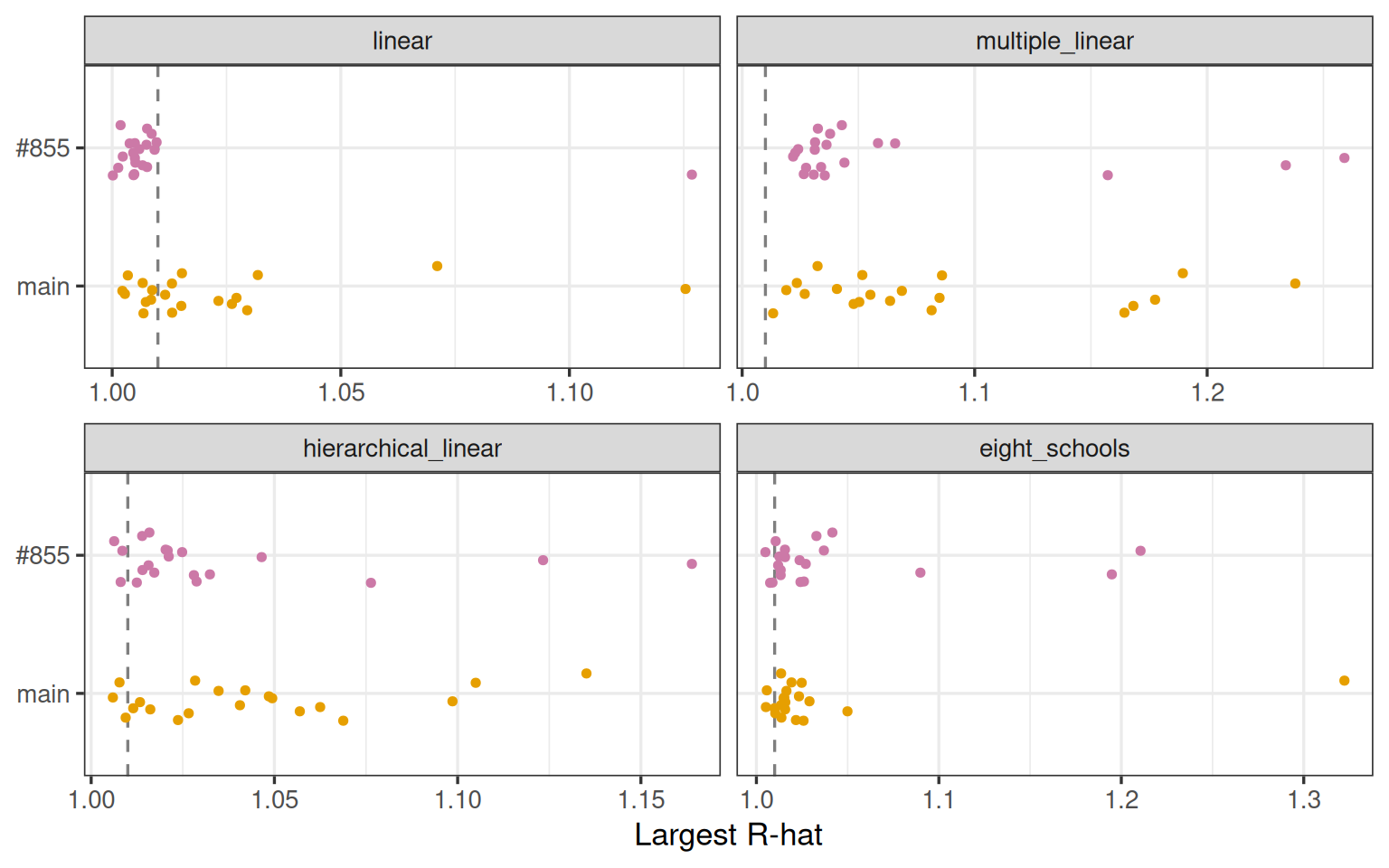
The largest R-hat (Vehtari et al. 2021) of each run, over its parameters. Above 1.01, the chains have not mixed well enough for their ESS to be trusted.

Code
ggplot(efficiency, aes(x = largest_rhat, y = version, colour = version)) +
  geom_vline(xintercept = 1.01, linetype = "dashed", colour = "grey50") +
  geom_point(
    position = position_jitter(width = 0, height = 0.2, seed = 2026),
    size = 1.2
  ) +
  scale_colour_manual(values = colours, guide = "none") +
  facet_wrap(vars(model), ncol = 2, scales = "free_x") +
  labs(x = "Largest R-hat", y = NULL)

Each small dot is one session’s run. The dashed line is at 1.01.
Code
# for each model and version, the median run's largest R-hat, the highest, and
# how many runs are above 1.01
convergence <- efficiency |>
  group_by(model, version) |>
  summarise(
    `median largest R-hat` = median(largest_rhat),
    `highest` = max(largest_rhat),
    `runs above 1.01` = paste(sum(largest_rhat > 1.01), "of", n()),
    .groups = "drop"
  )
capped <- efficiency |> filter(smallest_ess_capped)
knitr::kable(convergence, digits = 3)
model version median largest R-hat highest runs above 1.01
linear main 1.013 1.125 12 of 20
linear #855 1.005 1.127 1 of 20
multiple_linear main 1.059 1.238 20 of 20
multiple_linear #855 1.035 1.259 20 of 20
hierarchical_linear main 1.038 1.135 17 of 20
hierarchical_linear #855 1.021 1.164 17 of 20
eight_schools main 1.016 1.322 17 of 20
eight_schools #855 1.020 1.211 17 of 20

With 4 chains of 2,000 sampler iterations, the median run’s largest R-hat is 1.01 to 1.06 over the models and versions, and the highest is 1.32, so one run’s smallest ESS is a rough estimate. The posterior package capped 0 ESS estimates at S × log10(S) for S draws, which anticorrelated draws reach, and 0 runs had a capped estimate as their smallest bulk ESS.

Table: every run
Code
efficiency |>
  select(
    session,
    version,
    model,
    seconds,
    epsilon,
    smallest_ess_bulk,
    smallest_ess_tail,
    largest_rhat,
    ess_per_iteration,
    ess_per_second
  ) |>
  dt_table()

Session details

Code
first_session <- runs |> filter(session == sessions[[1]]$session)
session_info_of <- function(version) {
  first_session$results[[match(version, first_session$version)]]$session_info
}
sessioninfo::session_info() for main
Code
session_info_of("main")
─ Session info ───────────────────────────────────────────────────────────────
 setting  value
 version  R version 4.6.1 (2026-06-24)
 os       macOS Tahoe 26.5.2
 system   aarch64, darwin23
 ui       X11
 language (EN)
 collate  en_AU.UTF-8
 ctype    en_AU.UTF-8
 tz       Australia/Hobart
 date     2026-10-13
 pandoc   3.10 @ /opt/homebrew/bin/pandoc
 quarto   1.9.36 @ /usr/local/bin/quarto

─ Packages ───────────────────────────────────────────────────────────────────
 package        * version    date (UTC) lib source
 abind            1.4-8      2024-09-12 [1] CRAN (R 4.6.0)
 backports        1.5.1      2026-04-03 [1] CRAN (R 4.6.0)
 base64enc        0.1-6      2026-02-02 [1] CRAN (R 4.6.0)
 bench          * 1.1.4      2025-01-16 [3] CRAN (R 4.6.0)
 callr            3.8.0      2026-06-05 [1] CRAN (R 4.6.0)
 checkmate        2.3.4      2026-02-03 [2] CRAN (R 4.6.0)
 cli              3.6.6      2026-04-09 [1] CRAN (R 4.6.0)
 coda             0.19-4.1   2024-01-31 [1] CRAN (R 4.6.0)
 codetools        0.2-20     2024-03-31 [3] CRAN (R 4.6.1)
 crayon           1.5.3      2024-06-20 [1] CRAN (R 4.6.0)
 digest           0.6.39     2025-11-19 [1] CRAN (R 4.6.0)
 distributional   0.9.0      2026-09-08 [2] CRAN (R 4.6.1)
 future           1.76.0     2026-09-24 [1] CRAN (R 4.6.1)
 generics         0.1.4      2025-05-09 [2] CRAN (R 4.6.0)
 globals          0.20.0     2026-10-11 [1] CRAN (R 4.6.1)
 glue             1.8.1      2026-04-17 [1] CRAN (R 4.6.0)
 greta          * 0.6.0.9000 2026-10-12 [1] Github (greta-dev/greta@7301562)
 hms              1.1.4      2025-10-17 [1] CRAN (R 4.6.0)
 jsonlite         2.0.0      2025-03-27 [1] CRAN (R 4.6.0)
 lattice          0.23-1     2026-08-12 [3] CRAN (R 4.6.1)
 lifecycle        1.0.5      2026-01-08 [1] CRAN (R 4.6.0)
 listenv          1.1.0      2026-10-04 [1] CRAN (R 4.6.1)
 magrittr         2.0.5      2026-04-04 [1] CRAN (R 4.6.0)
 Matrix           1.7-6      2026-07-25 [3] CRAN (R 4.6.1)
 parallelly       1.48.0     2026-06-29 [1] CRAN (R 4.6.1)
 pillar           1.11.1     2025-09-17 [2] CRAN (R 4.6.0)
 pkgconfig        2.0.3      2019-09-22 [1] CRAN (R 4.6.0)
 png              0.1-9      2026-03-15 [1] CRAN (R 4.6.0)
 posterior        1.7.0      2026-04-01 [2] CRAN (R 4.6.0)
 prettyunits      1.2.0      2023-09-24 [1] CRAN (R 4.6.0)
 processx         3.9.0      2026-04-22 [1] CRAN (R 4.6.0)
 progress         1.2.3      2023-12-06 [1] CRAN (R 4.6.0)
 R6               2.6.1      2025-02-15 [1] CRAN (R 4.6.0)
 Rcpp             1.1.2      2026-07-05 [1] CRAN (R 4.6.1)
 reticulate       1.47.0     2026-09-03 [1] CRAN (R 4.6.1)
 rlang            1.3.0      2026-07-05 [1] CRAN (R 4.6.1)
 sessioninfo      1.2.4      2026-06-04 [3] CRAN (R 4.6.0)
 tensorA          0.36.2.1   2023-12-13 [2] CRAN (R 4.6.0)
 tensorflow       2.20.0     2025-08-22 [1] CRAN (R 4.6.0)
 tfautograph      0.3.2      2021-09-17 [1] CRAN (R 4.6.0)
 tfruns           1.5.4      2025-08-20 [1] CRAN (R 4.6.0)
 tibble           3.3.1      2026-01-11 [2] CRAN (R 4.6.0)
 vctrs            0.7.3      2026-04-11 [1] CRAN (R 4.6.0)
 whisker          0.4.1      2022-12-05 [1] CRAN (R 4.6.0)
 withr            3.0.3      2026-06-19 [1] CRAN (R 4.6.0)

 [1] /private/var/folders/cz/hrp33k3s0jlcb_gg9snlqh580000gq/T/RtmpmBvD0v/file62342adbfa5d
 [2] /Users/nick_1/Library/R/arm64/4.6/library
 [3] /Library/Frameworks/R.framework/Versions/4.6/Resources/library
 * ── Packages attached to the search path.

─ Python configuration ───────────────────────────────────────────────────────
 /Users/nick_1/.cache/uv/archive-v0/o_K93ThG1GwhxnXh80Txm/bin/python
 /Users/nick_1/.local/share/uv/python/cpython-3.12.13-macos-aarch64-none/lib/lib/libpython3.12.dylib
 /Users/nick_1/.cache/uv/archive-v0/o_K93ThG1GwhxnXh80Txm:/Users/nick_1/.cache/uv/archive-v0/o_K93ThG1GwhxnXh80Txm
 /Users/nick_1/.local/share/uv/python/cpython-3.12.13-macos-aarch64-none/lib/python312.zip:/Users/nick_1/.local/share/uv/python/cpython-3.12.13-macos-aarch64-none/lib/python3.12:/Users/nick_1/.local/share/uv/python/cpython-3.12.13-macos-aarch64-none/lib/python3.12/lib-dynload:/Users/nick_1/.cache/uv/archive-v0/o_K93ThG1GwhxnXh80Txm/lib/python3.12/site-packages
 /Users/nick_1/.cache/uv/archive-v0/o_K93ThG1GwhxnXh80Txm
 /Users/nick_1/.cache/uv/archive-v0/o_K93ThG1GwhxnXh80Txm
 /Users/nick_1/.local/share/uv/python/cpython-3.12.13-macos-aarch64-none
 /Users/nick_1/.cache/uv/archive-v0/o_K93ThG1GwhxnXh80Txm
 /Users/nick_1/.cache/uv/archive-v0/o_K93ThG1GwhxnXh80Txm/bin/activate_this.py
 /Users/nick_1/.cache/uv/archive-v0/o_K93ThG1GwhxnXh80Txm/bin/python
 /Users/nick_1/.local/share/uv/python/cpython-3.12.13-macos-aarch64-none/bin/python3.12
 3.12.13 (main, Mar 20 2026, 00:20:20) [Clang 22.1.1 ]
 3, 12
 64bit
 FALSE
 False
 /Users/nick_1/.cache/uv/archive-v0/o_K93ThG1GwhxnXh80Txm/lib/python3.12/site-packages/numpy, 2                                                                                          , 5                                                                                          , 3                                                                                          
 tensorflow
 /Users/nick_1/.cache/uv/archive-v0/o_K93ThG1GwhxnXh80Txm/lib/python3.12/site-packages/tensorflow
 TRUE
 /Users/nick_1/.cache/uv/archive-v0/o_K93ThG1GwhxnXh80Txm/bin/python
 py_require()
 TRUE

──────────────────────────────────────────────────────────────────────────────
sessioninfo::session_info() for #855
Code
session_info_of("#855")
─ Session info ───────────────────────────────────────────────────────────────
 setting  value
 version  R version 4.6.1 (2026-06-24)
 os       macOS Tahoe 26.5.2
 system   aarch64, darwin23
 ui       X11
 language (EN)
 collate  en_AU.UTF-8
 ctype    en_AU.UTF-8
 tz       Australia/Hobart
 date     2026-10-13
 pandoc   3.10 @ /opt/homebrew/bin/pandoc
 quarto   1.9.36 @ /usr/local/bin/quarto

─ Packages ───────────────────────────────────────────────────────────────────
 package        * version    date (UTC) lib source
 abind            1.4-8      2024-09-12 [1] CRAN (R 4.6.0)
 backports        1.5.1      2026-04-03 [1] CRAN (R 4.6.0)
 base64enc        0.1-6      2026-02-02 [1] CRAN (R 4.6.0)
 bench          * 1.1.4      2025-01-16 [3] CRAN (R 4.6.0)
 callr            3.8.0      2026-06-05 [1] CRAN (R 4.6.0)
 checkmate        2.3.4      2026-02-03 [2] CRAN (R 4.6.0)
 cli              3.6.6      2026-04-09 [1] CRAN (R 4.6.0)
 coda             0.19-4.1   2024-01-31 [1] CRAN (R 4.6.0)
 codetools        0.2-20     2024-03-31 [3] CRAN (R 4.6.1)
 crayon           1.5.3      2024-06-20 [1] CRAN (R 4.6.0)
 digest           0.6.39     2025-11-19 [1] CRAN (R 4.6.0)
 distributional   0.9.0      2026-09-08 [2] CRAN (R 4.6.1)
 future           1.76.0     2026-09-24 [1] CRAN (R 4.6.1)
 generics         0.1.4      2025-05-09 [2] CRAN (R 4.6.0)
 globals          0.20.0     2026-10-11 [1] CRAN (R 4.6.1)
 glue             1.8.1      2026-04-17 [1] CRAN (R 4.6.0)
 greta          * 0.6.0.9000 2026-10-12 [1] Github (greta-dev/greta@f6df006)
 hms              1.1.4      2025-10-17 [1] CRAN (R 4.6.0)
 jsonlite         2.0.0      2025-03-27 [1] CRAN (R 4.6.0)
 lattice          0.23-1     2026-08-12 [3] CRAN (R 4.6.1)
 lifecycle        1.0.5      2026-01-08 [1] CRAN (R 4.6.0)
 listenv          1.1.0      2026-10-04 [1] CRAN (R 4.6.1)
 magrittr         2.0.5      2026-04-04 [1] CRAN (R 4.6.0)
 Matrix           1.7-6      2026-07-25 [3] CRAN (R 4.6.1)
 parallelly       1.48.0     2026-06-29 [1] CRAN (R 4.6.1)
 pillar           1.11.1     2025-09-17 [2] CRAN (R 4.6.0)
 pkgconfig        2.0.3      2019-09-22 [1] CRAN (R 4.6.0)
 png              0.1-9      2026-03-15 [1] CRAN (R 4.6.0)
 posterior        1.7.0      2026-04-01 [2] CRAN (R 4.6.0)
 prettyunits      1.2.0      2023-09-24 [1] CRAN (R 4.6.0)
 processx         3.9.0      2026-04-22 [1] CRAN (R 4.6.0)
 progress         1.2.3      2023-12-06 [1] CRAN (R 4.6.0)
 R6               2.6.1      2025-02-15 [1] CRAN (R 4.6.0)
 Rcpp             1.1.2      2026-07-05 [1] CRAN (R 4.6.1)
 reticulate       1.47.0     2026-09-03 [1] CRAN (R 4.6.1)
 rlang            1.3.0      2026-07-05 [1] CRAN (R 4.6.1)
 sessioninfo      1.2.4      2026-06-04 [3] CRAN (R 4.6.0)
 tensorA          0.36.2.1   2023-12-13 [2] CRAN (R 4.6.0)
 tensorflow       2.20.0     2025-08-22 [1] CRAN (R 4.6.0)
 tfautograph      0.3.2      2021-09-17 [1] CRAN (R 4.6.0)
 tfruns           1.5.4      2025-08-20 [1] CRAN (R 4.6.0)
 tibble           3.3.1      2026-01-11 [2] CRAN (R 4.6.0)
 vctrs            0.7.3      2026-04-11 [1] CRAN (R 4.6.0)
 whisker          0.4.1      2022-12-05 [1] CRAN (R 4.6.0)
 withr            3.0.3      2026-06-19 [1] CRAN (R 4.6.0)

 [1] /private/var/folders/cz/hrp33k3s0jlcb_gg9snlqh580000gq/T/RtmpmBvD0v/file6234501205a6
 [2] /Users/nick_1/Library/R/arm64/4.6/library
 [3] /Library/Frameworks/R.framework/Versions/4.6/Resources/library
 * ── Packages attached to the search path.

─ Python configuration ───────────────────────────────────────────────────────
 /Users/nick_1/.cache/uv/archive-v0/o_K93ThG1GwhxnXh80Txm/bin/python
 /Users/nick_1/.local/share/uv/python/cpython-3.12.13-macos-aarch64-none/lib/lib/libpython3.12.dylib
 /Users/nick_1/.cache/uv/archive-v0/o_K93ThG1GwhxnXh80Txm:/Users/nick_1/.cache/uv/archive-v0/o_K93ThG1GwhxnXh80Txm
 /Users/nick_1/.local/share/uv/python/cpython-3.12.13-macos-aarch64-none/lib/python312.zip:/Users/nick_1/.local/share/uv/python/cpython-3.12.13-macos-aarch64-none/lib/python3.12:/Users/nick_1/.local/share/uv/python/cpython-3.12.13-macos-aarch64-none/lib/python3.12/lib-dynload:/Users/nick_1/.cache/uv/archive-v0/o_K93ThG1GwhxnXh80Txm/lib/python3.12/site-packages
 /Users/nick_1/.cache/uv/archive-v0/o_K93ThG1GwhxnXh80Txm
 /Users/nick_1/.cache/uv/archive-v0/o_K93ThG1GwhxnXh80Txm
 /Users/nick_1/.local/share/uv/python/cpython-3.12.13-macos-aarch64-none
 /Users/nick_1/.cache/uv/archive-v0/o_K93ThG1GwhxnXh80Txm
 /Users/nick_1/.cache/uv/archive-v0/o_K93ThG1GwhxnXh80Txm/bin/activate_this.py
 /Users/nick_1/.cache/uv/archive-v0/o_K93ThG1GwhxnXh80Txm/bin/python
 /Users/nick_1/.local/share/uv/python/cpython-3.12.13-macos-aarch64-none/bin/python3.12
 3.12.13 (main, Mar 20 2026, 00:20:20) [Clang 22.1.1 ]
 3, 12
 64bit
 FALSE
 False
 /Users/nick_1/.cache/uv/archive-v0/o_K93ThG1GwhxnXh80Txm/lib/python3.12/site-packages/numpy, 2                                                                                          , 5                                                                                          , 3                                                                                          
 tensorflow
 /Users/nick_1/.cache/uv/archive-v0/o_K93ThG1GwhxnXh80Txm/lib/python3.12/site-packages/tensorflow
 TRUE
 /Users/nick_1/.cache/uv/archive-v0/o_K93ThG1GwhxnXh80Txm/bin/python
 py_require()
 TRUE

──────────────────────────────────────────────────────────────────────────────

References

Girolami, Mark, and Ben Calderhead. 2011. “Riemann Manifold Langevin and Hamiltonian Monte Carlo Methods.” Journal of the Royal Statistical Society: Series B (Statistical Methodology) 73 (2): 123–214. https://doi.org/10.1111/j.1467-9868.2010.00765.x.
Hoffman, Matthew D., and Andrew Gelman. 2014. “The No-U-Turn Sampler: Adaptively Setting Path Lengths in Hamiltonian Monte Carlo.” Journal of Machine Learning Research 15 (47): 1593–623. https://jmlr.org/papers/v15/hoffman14a.html.
Vehtari, Aki, Andrew Gelman, Daniel Simpson, Bob Carpenter, and Paul-Christian Bürkner. 2021. “Rank-Normalization, Folding, and Localization: An Improved R̂ for Assessing Convergence of MCMC (with Discussion).” Bayesian Analysis 16 (2): 667–718. https://doi.org/10.1214/20-BA1221.