greta#843 (faster-hessians-i546): retracing and hessians

Building models, opt(), opt(hessian = TRUE) and mcmc() on greta 0.6.0 from CRAN, on main and on greta#843. greta#843 traces each model’s TensorFlow functions fewer times, and opt(hessian = TRUE) is much faster on it.

suppressPackageStartupMessages({
  library(dplyr)
  library(tidyr)
  library(ggplot2)
  library(bench)
  library(here)
})

post_path <- "posts/2026-10-05-retracing-i546"

# each `# ---- label ----` section of the scripts, shown below by its label
knitr::read_chunk(here(post_path, "benchmark.R"))
knitr::read_chunk(here(post_path, "run.R"))

# links to the scripts on GitHub, at the commit being rendered when GitHub
# Actions renders the site
github_ref <- Sys.getenv("GITHUB_SHA", "main")
github_file_url <- function(file) {
  paste0(
    "https://github.com/greta-dev/greta.benchmarks/blob/",
    github_ref,
    "/",
    post_path,
    "/",
    file
  )
}
# Quarto escapes the markdown in an inline `{r}` result unless it is wrapped
# in I(), so the link helpers return I()
file_link <- function(file) {
  I(paste0("[`", file, "`](", github_file_url(file), ")"))
}

# a link to the lines of a script's `# ---- label ----` section
section_link <- function(file, label) {
  lines <- readLines(here(post_path, file))
  headings <- grep("^# ---- .+ ----$", lines)
  start <- headings[lines[headings] == paste("# ----", label, "----")]
  end <- c(headings, length(lines) + 1)[match(start, headings) + 1] - 1
  while (end > start && !nzchar(trimws(lines[end]))) {
    end <- end - 1
  }
  I(paste0(
    "[`", label, "`](", github_file_url(file), "#L", start, "-L", end, ")"
  ))
}

# "CRAN, main and #843"
paste_and <- function(x) {
  if (length(x) <= 1) {
    return(x)
  }
  paste(paste(x[-length(x)], collapse = ", "), "and", x[length(x)])
}

# links to several sections of a script, as "a, b and c"
section_links <- function(file, labels) {
  links <- vapply(
    labels,
    \(label) as.character(section_link(file, label)),
    character(1)
  )
  I(paste_and(links))
}

# white panels, so the grey band in the agreement plot shows
theme_set(theme_bw())

sessions <- list.files(
  here(post_path, "results"),
  pattern = "^session-[0-9]+[.]rds$",
  full.names = TRUE
) |>
  lapply(readRDS)

versions <- sessions[[1]]$versions
version_levels <- names(versions)
version_colours <- setNames(
  c("#E69F00", "#56B4E9", "#009E73")[seq_along(version_levels)],
  version_levels
)
# the version this post is about: every ratio is against it
pr_version <- "#843"
bench_settings <- sessions[[1]]$results[[1]]$bench_settings
n_sessions <- length(sessions)

# one row per session and version, holding that version's results
runs <- lapply(sessions, function(session_file) {
  tibble(
    session = session_file$session,
    version = factor(names(session_file$results), levels = version_levels),
    position = match(names(session_file$results), session_file$order),
    results = unname(session_file$results)
  )
}) |>
  bind_rows()

model_levels <- names(runs$results[[1]]$build)
# benchmark.R's section labels spell each model with hyphens
model_labels <- gsub("_", "-", model_levels)

# a part of the results that is a table or a value per run, stacked, with the
# run it came from
stack_tables <- function(part) {
  pieces <- lapply(seq_len(nrow(runs)), function(i) {
    values <- runs$results[[i]][[part]]
    if (!is.data.frame(values)) {
      values <- tibble(value = values)
    }
    tibble(session = runs$session[i], version = runs$version[i], values)
  })
  bind_rows(pieces)
}

# a part of the results that is a bench_mark per model, or one per run,
# stacked into one bench_mark, with the run and model each came from
stack_marks <- function(part) {
  pieces <- list()
  for (i in seq_len(nrow(runs))) {
    marks <- runs$results[[i]][[part]]
    if (inherits(marks, "bench_mark")) {
      marks <- list(marks)
    }
    for (j in seq_along(marks)) {
      mark <- marks[[j]]
      mark$session <- runs$session[i]
      mark$version <- runs$version[i]
      mark$model <- if (is.null(names(marks))) NA_character_ else names(marks)[j]
      pieces[[length(pieces) + 1]] <- mark
    }
  }
  vctrs::vec_rbind(!!!pieces)
}

provenance <- stack_tables("provenance")
sampler_iterations_per_draw <- stack_tables("sampler_iterations_per_draw")
build_marks <- stack_marks("build")
opt_marks <- stack_marks("opt")
hessian_marks <- stack_marks("hessian")
hessian_retracing_warnings <- stack_tables("hessian_retracing_warnings")
mcmc_marks <- stack_marks("mcmc")
mcmc_tracing <- stack_tables("mcmc_tracing")

# one row per timed call: bench keeps every call's time in the `time` column
every_call <- function(marks) {
  marks |>
    as_tibble() |>
    select(session, version, model, time) |>
    mutate(call = lapply(time, seq_along)) |>
    unnest(c(time, call)) |>
    mutate(
      seconds = as.numeric(time),
      model = factor(model, levels = model_levels),
      .keep = "unused"
    )
}

# bench's own summary() of each mark, with the mean and longest of its calls
# added, all in seconds
bench_summary <- function(marks) {
  summaries <- summary(marks, filter_gc = FALSE)
  tibble(
    session = summaries$session,
    version = summaries$version,
    model = summaries$model,
    min = as.numeric(summaries$min),
    median = as.numeric(summaries$median),
    mean = vapply(marks$time, \(time) mean(as.numeric(time)), numeric(1)),
    max = vapply(marks$time, \(time) max(as.numeric(time)), numeric(1)),
    `itr/sec` = summaries$`itr/sec`,
    n_itr = summaries$n_itr,
    total_time = as.numeric(summaries$total_time)
  )
}

# each version's median call, from a table of every call
version_medians <- function(calls) {
  calls |>
    group_by(version) |>
    summarise(seconds = median(seconds))
}

# The first call on a model traces its TensorFlow functions; later calls on the
# same model reuse them.
label_calls <- function(call) {
  last <- max(call)
  later <- if (last == 2) {
    "second call on the same model"
  } else if (last == 3) {
    "calls 2 and 3 on the same model"
  } else {
    paste0("calls 2 to ", last, " on the same model")
  }
  factor(
    ifelse(call == 1, "first call on a new model", later),
    levels = c("first call on a new model", later)
  )
}

# three significant figures each, where format() would pad a vector to the
# decimal places of its smallest value; formatC() pads each to a common width,
# so the spaces are trimmed
format_number <- function(x) {
  trimws(formatC(signif(x, 3), format = "fg", digits = 3, big.mark = ","))
}

# "CRAN 10.6, main 11.2, #843 0.643"
versions_text <- function(version, value) {
  paste(paste(version, format_number(value)), collapse = ", ")
}

# a version's value, from a table with one row per version
value_of <- function(table, version_name, column = "seconds") {
  table[[column]][table$version == version_name]
}

# how many times as long as #843 a version takes, from a table of medians
times_as_long <- function(table, version_name) {
  format_number(value_of(table, version_name) / value_of(table, pr_version))
}

# "once", "twice" or "3 times"
times_word <- function(n) {
  ifelse(n == 1, "once", ifelse(n == 2, "twice", paste(n, "times")))
}

version_scale <- scale_colour_manual(values = version_colours, guide = "none")
version_fill <- scale_fill_manual(values = version_colours, guide = "none")
jitter <- position_jitter(width = 0, height = 0.2, seed = 2026)

# A raincloud for each version: the density of its calls above, their box plot
# in the middle, and every call as a dot below. The summaries are drawn first
# and faint, so the dots sit on top.
raincloud <- list(
  ggdist::stat_halfeye(
    aes(fill = version),
    width = 0.4,
    justification = -0.3,
    .width = 0,
    point_colour = NA,
    alpha = 0.3
  ),
  geom_boxplot(
    aes(fill = version),
    width = 0.25,
    outlier.shape = NA,
    alpha = 0.3
  ),
  # a fixed dot size, so a call looks the same size in every panel
  ggdist::stat_dots(
    aes(fill = version),
    side = "bottom",
    layout = "swarm",
    justification = 1.3,
    scale = 0.75,
    binwidth = unit(2.6, "mm"),
    overflow = "compress",
    colour = NA,
    alpha = 0.6
  ),
  version_scale,
  version_fill,
  theme_bw(base_size = 13)
)
raincloud_caption <- "Each dot is one call, from every session. Above the dots, the curve is the density of the calls and the box marks their median and quartiles."
session_caption <- "Each small dot is one session's second call. The large faint dot behind them is their mean."

# a searchable table, its numbers rounded for reading
dt_table <- function(data, digits = 3) {
  table <- DT::datatable(
    data,
    rownames = FALSE,
    filter = "top",
    options = list(pageLength = 10, autoWidth = TRUE)
  )
  decimal_columns <- names(data)[vapply(data, is.double, logical(1))]
  if (length(decimal_columns) == 0) {
    return(table)
  }
  DT::formatRound(table, decimal_columns, digits)
}

# a model's draws array is draws by chains by parameters
parameter_count <- function(name) {
  dim(runs$results[[1]]$mcmc_draws[[name]])[3]
}

# wide enough for a column of panels per parameter
draws_width <- function(name) {
  max(8, 1.6 * parameter_count(name))
}

# the opening's numbers: each version's median opt(hessian = TRUE) call, and
# how many times mcmc() traced each model's log density
opening_hessian <- version_medians(every_call(hessian_marks))
opening_traces <- mcmc_tracing |>
  group_by(version) |>
  summarise(
    traces = paste(times_word(sort(unique(log_prob_traces))), collapse = " or ")
  )

greta#843 traces each model’s log-density and trace-values functions once, whatever the batch size, and takes all of opt(hessian = TRUE)’s hessians in one graph build. This post compares it with greta 0.6.0 on CRAN and with main. On a model with twenty hessians, an opt(hessian = TRUE) call takes a median of 0.635 seconds on #843; CRAN takes 15.9 times as long, and main 18.6 times as long. In mcmc(), #843 traces each model’s log density once, where CRAN traces it twice and main twice.

How long does opt(hessian = TRUE) take?

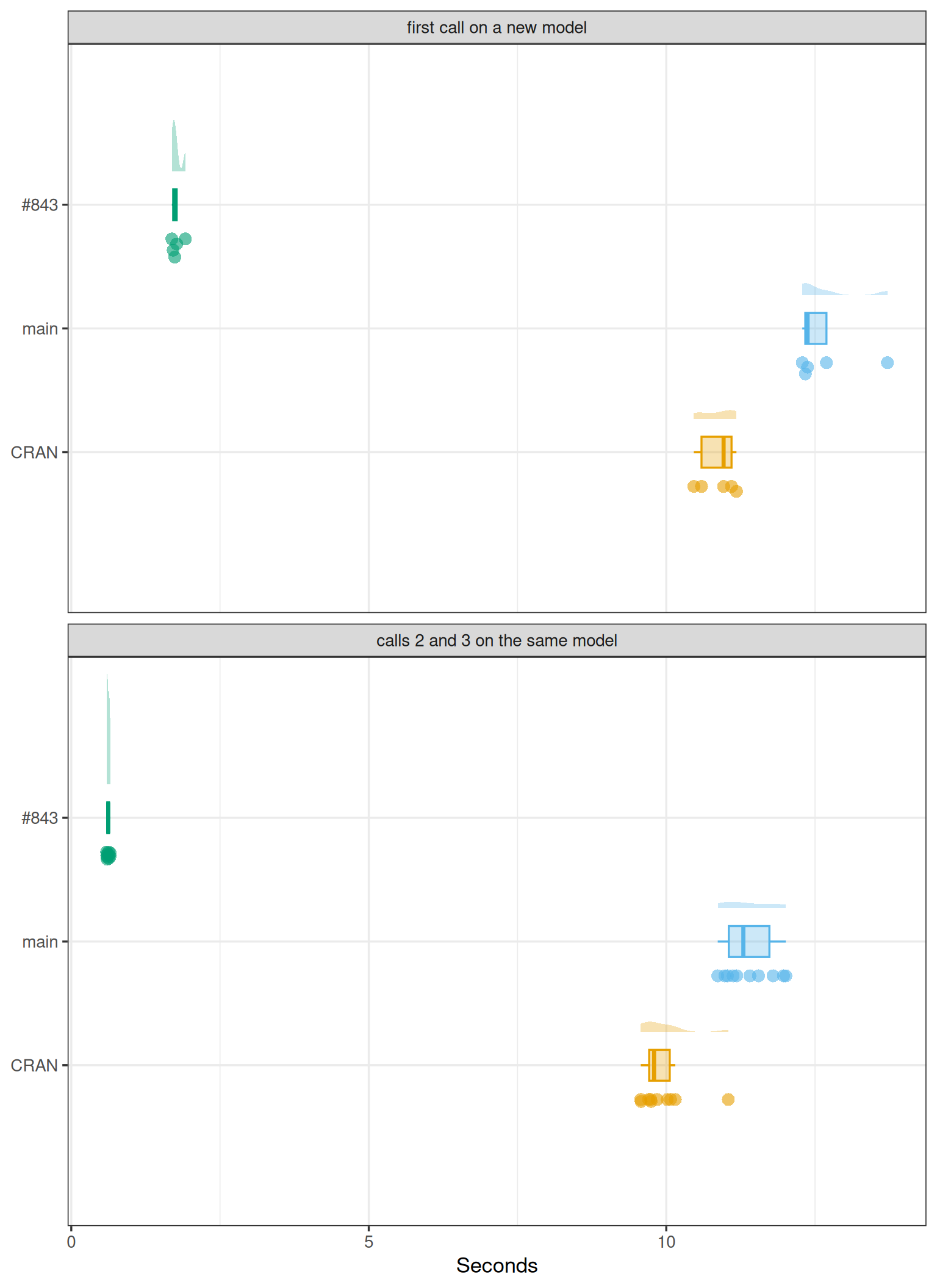
Each session called opt(hessian = TRUE) 3 times on the hessian model, whose twenty scalar parameters each need a hessian. The first call traces the model’s TensorFlow functions and later calls reuse them, so they are plotted apart.

hessian <- every_call(hessian_marks) |>
  select(-model) |>
  mutate(calls = label_calls(call))
hessian_summary <- bench_summary(hessian_marks) |>
  select(-model)

# each version's median first call, and its median later call
hessian_medians <- hessian |>
  group_by(version, first_call = call == 1) |>
  summarise(seconds = median(seconds), .groups = "drop")
hessian_first <- filter(hessian_medians, first_call)
hessian_later <- filter(hessian_medians, !first_call)

hessian_warning_counts <- hessian_retracing_warnings |>
  group_by(version) |>
  summarise(counts = paste(sort(unique(value)), collapse = " or "))

ggplot(hessian, aes(x = seconds, y = version, colour = version)) +
  raincloud +
  facet_wrap(~calls, ncol = 1) +
  labs(x = "Seconds", y = NULL)

Each dot is one call, from every session. Above the dots, the curve is the density of the calls and the box marks their median and quartiles.

Timed by benchmark.R’s bench-hessian section.

The median first call takes CRAN 11, main 12.4, #843 1.74 seconds, and the median later call CRAN 9.8, main 11.3, #843 0.621. So on later calls, CRAN takes 15.8 times as long as #843, and main 18.2 times as long. TensorFlow’s retracing warnings during each session’s calls, counted in the same section: CRAN 2, main 2, #843 0.

Table: bench’s summary() of every mark

dt_table(hessian_summary, digits = 4)

Table: every call

dt_table(hessian, digits = 4)

How many times does mcmc() trace a model?

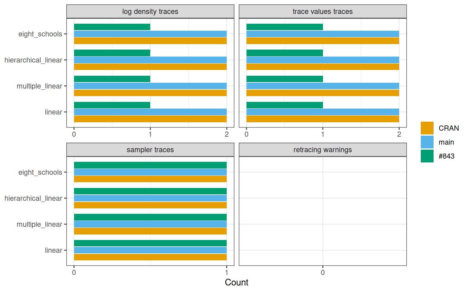
After both of a model’s mcmc() calls, each session asked each of the model’s TensorFlow functions how many times it had been traced, and counted the retracing warnings TensorFlow logged during the two calls.

tracing <- mcmc_tracing |>
  pivot_longer(
    c(retracing_warnings, ends_with("_traces")),
    names_to = "measure",
    values_to = "count"
  ) |>
  mutate(
    model = factor(model, levels = model_levels),
    measure = factor(
      measure,
      levels = c("log_prob_traces", "trace_values_traces", "sampler_traces", "retracing_warnings"),
      labels = c("log density traces", "trace values traces", "sampler traces", "retracing warnings")
    )
  )

# whether every session gave the same count, so one bar can stand for them all
counts_per_session <- tracing |>
  group_by(version, model, measure) |>
  summarise(distinct_counts = n_distinct(count), .groups = "drop")
same_in_every_session <- all(counts_per_session$distinct_counts == 1)

# how many times a version traced a function, over every model and session
traced <- function(measure_name, version_name) {
  counts <- tracing$count[
    tracing$measure == measure_name & tracing$version == version_name
  ]
  paste(times_word(sort(unique(counts))), collapse = " or ")
}

Each count was the same in all 5 sessions, so each bar is that count.

tracing_plot <- ggplot(tracing, aes(x = count, y = model)) +
  scale_x_continuous(breaks = \(limits) unique(floor(pretty(limits)))) +
  facet_wrap(~measure, ncol = 2, scales = "free_x") +
  labs(x = "Count", y = NULL, fill = NULL, colour = NULL)

# bars are filled and dots coloured, so each draws only the scale it uses
if (same_in_every_session) {
  tracing_plot +
    geom_col(
      aes(fill = version),
      data = distinct(tracing, version, model, measure, count),
      position = position_dodge(width = 0.8),
      width = 0.75
    ) +
    scale_fill_manual(values = version_colours)
} else {
  tracing_plot +
    geom_point(aes(colour = version), position = position_dodge(width = 0.8)) +
    scale_colour_manual(values = version_colours)
}

Counted by benchmark.R’s mcmc-tracing section, with the helpers in its benchmark-helpers section.

On #843, each model’s log density is traced once and its trace values once; on CRAN, twice and twice; on main, twice and twice. TensorFlow logged 0 retracing warnings during mcmc(), over every version, model and session.

Table: every count

dt_table(tracing)

How long does mcmc() take?

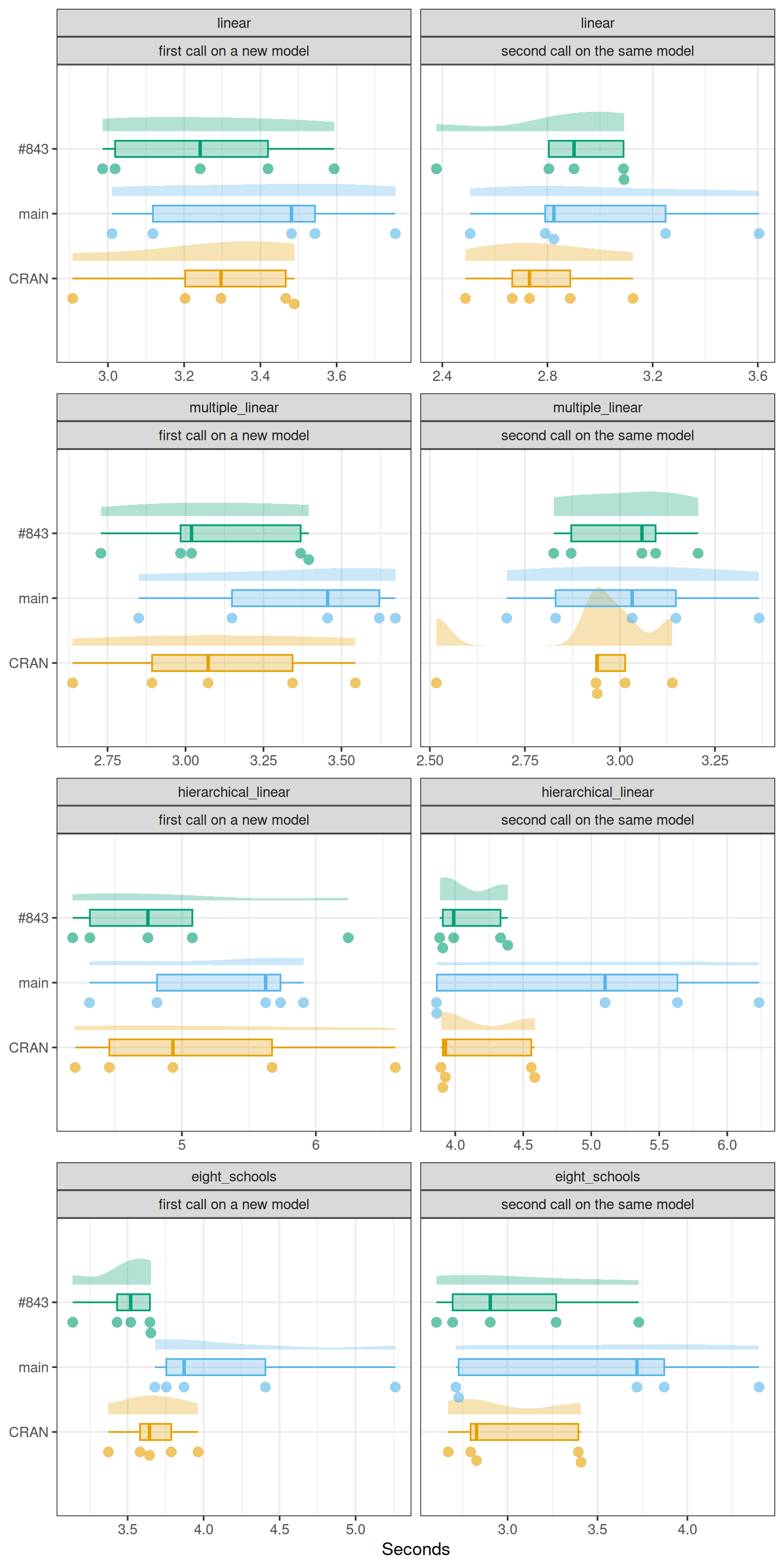
Each session called mcmc() twice on each model, with 1000 warmup and 1000 kept draws on each of 4 chains: first on a new model, which traces its TensorFlow functions, then on the same model again.

mcmc_timings <- every_call(mcmc_marks) |>
  mutate(calls = label_calls(call))
mcmc_summary <- bench_summary(mcmc_marks)
mcmc_medians <- version_medians(mcmc_timings)

ggplot(mcmc_timings, aes(x = seconds, y = version, colour = version)) +
  raincloud +
  facet_wrap(vars(model, calls), ncol = 2, scales = "free_x") +
  labs(x = "Seconds", y = NULL)

Each dot is one call, from every session. Above the dots, the curve is the density of the calls and the box marks their median and quartiles.

Timed by benchmark.R’s bench-mcmc-linear, bench-mcmc-multiple-linear, bench-mcmc-hierarchical-linear and bench-mcmc-eight-schools sections.

Over all models and both calls, the median call takes 3.26 seconds on #843; CRAN takes 1.03 times as long, and main 1.12 times as long.

Table: bench’s summary() of every mark

dt_table(mcmc_summary, digits = 4)

Table: every call

dt_table(mcmc_timings, digits = 4)

How many effective draws per second does mcmc() give?

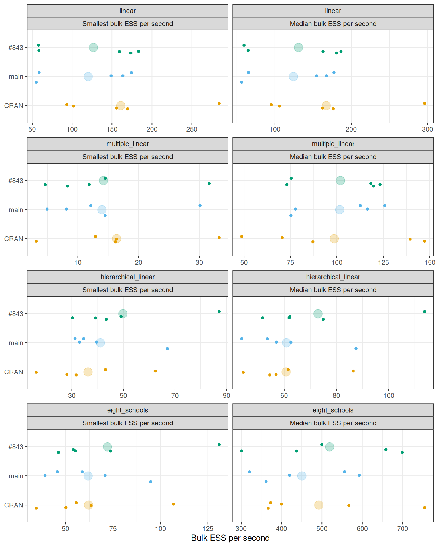
Efficiency is the bulk effective sample size (ESS) per second, the time-normalised ESS of Girolami and Calderhead (2011), for the parameter with the smallest bulk ESS, as Hoffman and Gelman (2014) report, and for the median parameter (Vehtari et al. 2021). It uses every draw of each model’s second mcmc() call, and that call’s seconds, warmup included.

posterior <- lapply(seq_len(nrow(runs)), function(i) {
  draws <- runs$results[[i]]$mcmc_draws
  lapply(names(draws), function(model_name) {
    tibble(
      session = runs$session[i],
      version = runs$version[i],
      model = model_name,
      posterior::summarise_draws(
        draws[[model_name]],
        "mean",
        "sd",
        "mcse_mean",
        "rhat",
        "ess_bulk",
        "ess_tail"
      )
    )
  }) |>
    bind_rows()
}) |>
  bind_rows() |>
  mutate(model = factor(model, levels = model_levels))

second_calls <- mcmc_timings |>
  filter(call == 2) |>
  select(session, version, model, seconds)

efficiency <- posterior |>
  group_by(session, version, model) |>
  summarise(
    smallest_ess_bulk = min(ess_bulk),
    median_ess_bulk = median(ess_bulk),
    .groups = "drop"
  ) |>
  left_join(second_calls, by = c("session", "version", "model")) |>
  mutate(
    smallest_ess_per_second = smallest_ess_bulk / seconds,
    median_ess_per_second = median_ess_bulk / seconds
  )

efficiency_means <- efficiency |>
  group_by(model, version) |>
  summarise(
    smallest_ess_per_second = mean(smallest_ess_per_second),
    median_ess_per_second = mean(median_ess_per_second),
    .groups = "drop"
  )

# one row per session, model, version and measure, for one panel per measure
efficiency_measures <- c(
  smallest_ess_per_second = "Smallest bulk ESS per second",
  median_ess_per_second = "Median bulk ESS per second"
)
longer_efficiency <- function(data) {
  data |>
    pivot_longer(
      all_of(names(efficiency_measures)),
      names_to = "measure",
      values_to = "ess_per_second"
    ) |>
    mutate(
      measure = factor(
        efficiency_measures[measure],
        levels = efficiency_measures
      )
    )
}

# #843's mean smallest bulk ESS per second over another version's, per model
efficiency_ratios <- efficiency_means |>
  group_by(model) |>
  summarise(
    of_cran = smallest_ess_per_second[version == pr_version] /
      smallest_ess_per_second[version == "CRAN"],
    of_main = smallest_ess_per_second[version == pr_version] /
      smallest_ess_per_second[version == "main"]
  )

ggplot(
  longer_efficiency(efficiency),
  aes(x = ess_per_second, y = version, colour = version)
) +
  geom_point(
    data = longer_efficiency(efficiency_means),
    size = 5,
    alpha = 0.25
  ) +
  geom_point(position = jitter, size = 1.2) +
  version_scale +
  facet_wrap(vars(model, measure), ncol = 2, scales = "free_x") +
  labs(x = "Bulk ESS per second", y = NULL)

Each small dot is one session’s second call. The large faint dot behind them is their mean.

The draws were kept by benchmark.R’s mcmc-draws section, and the calls timed by its bench-mcmc-linear, bench-mcmc-multiple-linear, bench-mcmc-hierarchical-linear and bench-mcmc-eight-schools sections.

Depending on the model, #843 gives between 0.787 and 1.37 times CRAN’s mean smallest bulk ESS per second, and between 1.02 and 1.21 times main’s.

Table: mean ESS per second

dt_table(efficiency_means, digits = 1)

Table: every session

dt_table(efficiency, digits = 1)

How long does opt() take?

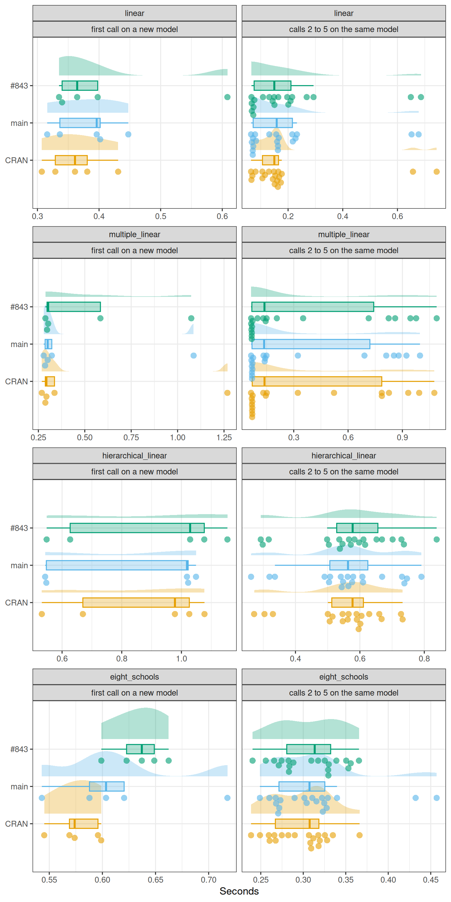
Each session called opt() 5 times on each model, built once for it. The first call traces the model’s TensorFlow functions and later calls reuse them.

opt_timings <- every_call(opt_marks) |>
  mutate(calls = label_calls(call))
opt_summary <- bench_summary(opt_marks)
opt_medians <- version_medians(opt_timings)

ggplot(opt_timings, aes(x = seconds, y = version, colour = version)) +
  raincloud +
  facet_wrap(vars(model, calls), ncol = 2, scales = "free_x") +
  labs(x = "Seconds", y = NULL)

Each dot is one call, from every session. Above the dots, the curve is the density of the calls and the box marks their median and quartiles.

Timed by benchmark.R’s bench-opt-linear, bench-opt-multiple-linear, bench-opt-hierarchical-linear and bench-opt-eight-schools sections.

Over all models and calls, the median call takes 0.329 seconds on #843; CRAN takes 0.965 times as long, and main 0.978 times as long.

Table: bench’s summary() of every mark

dt_table(opt_summary, digits = 4)

Table: every call

dt_table(opt_timings, digits = 4)

How long does building a model take?

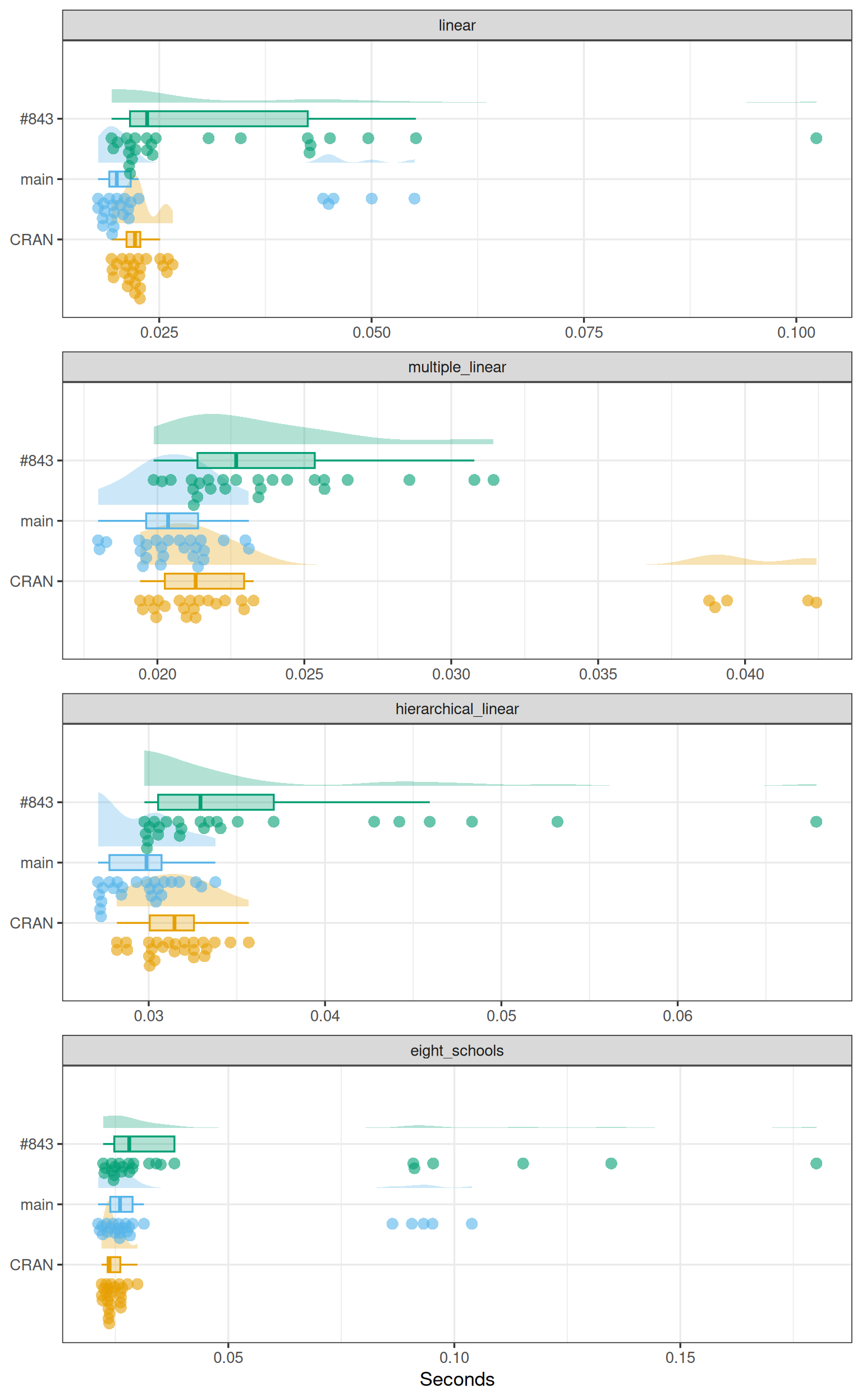
Each session built each model 5 times: creating its greta arrays and calling model().

build <- every_call(build_marks)
build_summary <- bench_summary(build_marks)
build_medians <- version_medians(build)

ggplot(build, aes(x = seconds, y = version, colour = version)) +
  raincloud +
  facet_wrap(~model, ncol = 1, scales = "free_x") +
  labs(x = "Seconds", y = NULL)

Each dot is one call, from every session. Above the dots, the curve is the density of the calls and the box marks their median and quartiles.

Timed by benchmark.R’s bench-build-linear, bench-build-multiple-linear, bench-build-hierarchical-linear and bench-build-eight-schools sections.

Over all models, the median build takes 0.028 seconds on #843; CRAN takes 0.842 times as long, and main 0.828 times as long.

Table: bench’s summary() of every mark

dt_table(build_summary, digits = 4)

Table: every call

dt_table(build, digits = 4)

Do the versions sample the same posterior?

For each parameter, each version’s posterior means and their Monte Carlo standard errors (MCSE) are pooled over its sessions, and two versions’ pooled means are compared by

\[ z = \frac{\bar\theta_{\text{b}} - \bar\theta_{\text{a}}}{\sqrt{\text{se}^2_{\text{a}} + \text{se}^2_{\text{b}}}}, \]

so a difference can be told apart from Monte Carlo noise (Vehtari et al. 2021; Magnusson et al. 2025). Each session has a seed of its own, so the sessions are independent, and a version’s pooled standard error is \(\sqrt{\sum \text{mcse}^2} / n\) over its \(n\) sessions. If both versions sample the same posterior, each \(z\) is close to a standard normal draw; two versions that return the same draws from the same seed give a \(z\) of zero.

pooled <- posterior |>
  group_by(version, model, variable) |>
  summarise(
    sessions = n(),
    mean = mean(mean),
    se = sqrt(sum(mcse_mean^2)) / n(),
    .groups = "drop"
  )

pairs <- utils::combn(version_levels, 2)
agreement <- lapply(seq_len(ncol(pairs)), function(i) {
  reference <- filter(pooled, version == pairs[1, i])
  compared <- filter(pooled, version == pairs[2, i])
  inner_join(reference, compared, by = c("model", "variable"), suffix = c("_a", "_b")) |>
    mutate(
      comparison = paste(pairs[2, i], "vs", pairs[1, i]),
      z = (mean_b - mean_a) / sqrt(se_a^2 + se_b^2)
    )
}) |>
  bind_rows() |>
  mutate(comparison = factor(comparison, levels = unique(comparison)))

# the band all of a comparison's z fall inside with probability 0.95 when both
# versions sample the same posterior: a Bonferroni bound over its parameters
parameters_compared <- n_distinct(paste(agreement$model, agreement$variable))
band <- qnorm(1 - 0.05 / (2 * parameters_compared))

outside_band <- agreement |>
  group_by(comparison) |>
  summarise(outside = sum(abs(z) > band), largest_abs_z = max(abs(z)))

# whether two versions returned the same draws in every session
draws_identical <- function(pair) {
  all(vapply(
    unique(runs$session),
    function(session_number) {
      first <- runs$results[[which(runs$session == session_number & runs$version == pair[1])]]
      second <- runs$results[[which(runs$session == session_number & runs$version == pair[2])]]
      identical(first$mcmc_draws, second$mcmc_draws)
    },
    logical(1)
  ))
}
identical_pairs <- Filter(
  draws_identical,
  utils::combn(version_levels, 2, simplify = FALSE)
)
identical_text <- if (length(identical_pairs) == 0) {
  "No two versions returned the same draws."
} else {
  paste0(
    vapply(identical_pairs, \(pair) paste(pair, collapse = "'s and "), character(1)),
    "'s draws are identical in every session.",
    collapse = " "
  )
}

ggplot(agreement, aes(x = z, y = model)) +
  annotate(
    "rect",
    xmin = -band,
    xmax = band,
    ymin = -Inf,
    ymax = Inf,
    fill = "grey80",
    alpha = 0.5
  ) +
  geom_point(position = jitter, alpha = 0.7) +
  facet_wrap(~comparison, ncol = 1) +
  labs(x = "z", y = NULL)

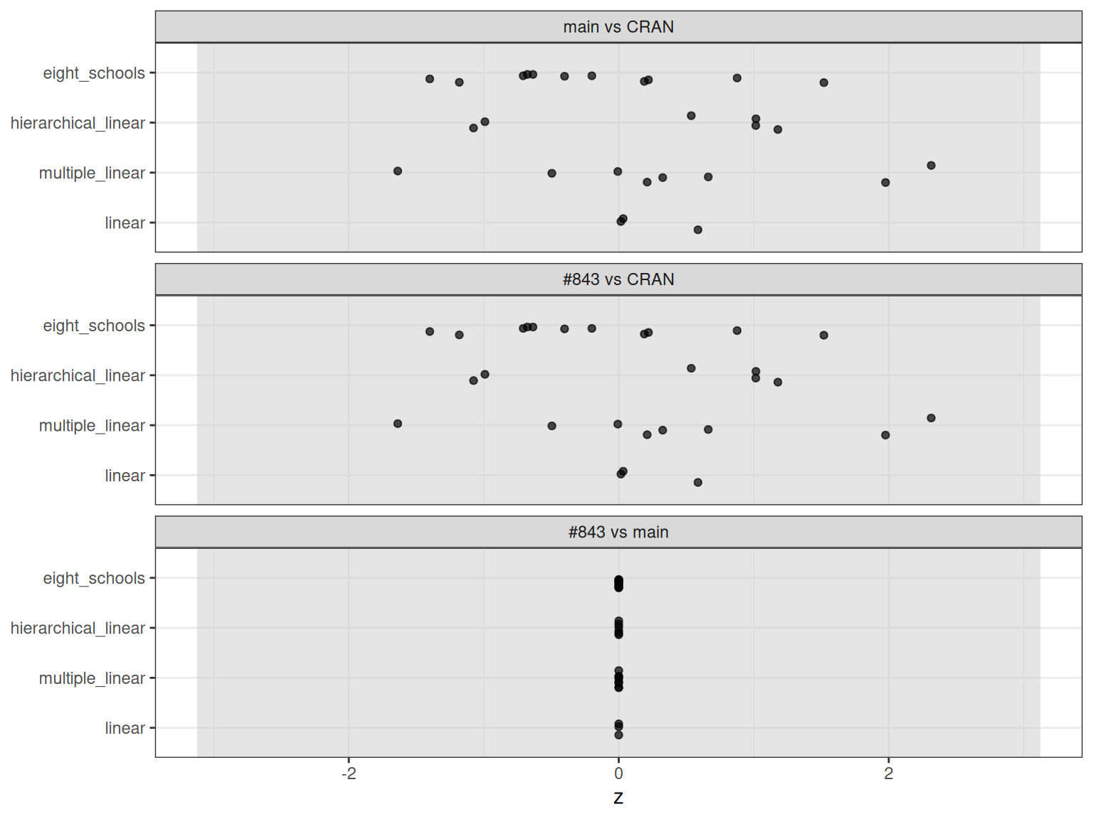
Each dot is one parameter. The grey band is where every parameter’s z falls, with probability at least 0.95, when both versions sample the same posterior.

From the draws of each model’s second mcmc() call, kept by benchmark.R’s mcmc-draws section.

The grey band is \(\pm\) 3.12, a Bonferroni bound over the 28 parameters. Parameters outside it, per comparison: main vs CRAN 0, #843 vs CRAN 0, #843 vs main 0. main’s and #843’s draws are identical in every session.

Table: largest |z| per comparison and model

agreement |>
  group_by(comparison, model) |>
  summarise(
    parameters = n(),
    largest_abs_z = max(abs(z)),
    parameter = variable[which.max(abs(z))],
    .groups = "drop"
  ) |>
  dt_table(digits = 2)

Table: every parameter

agreement |>
  select(comparison, model, variable, mean_a, se_a, mean_b, se_b, z) |>
  dt_table()

Traceplots

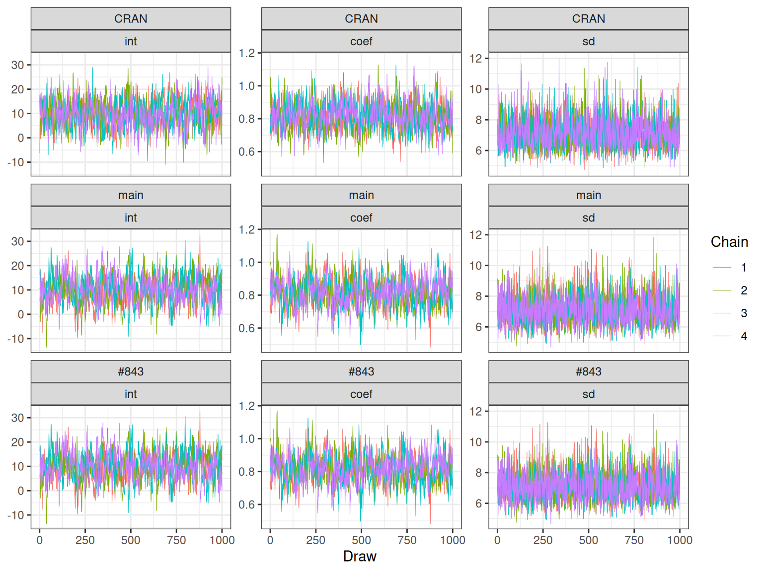
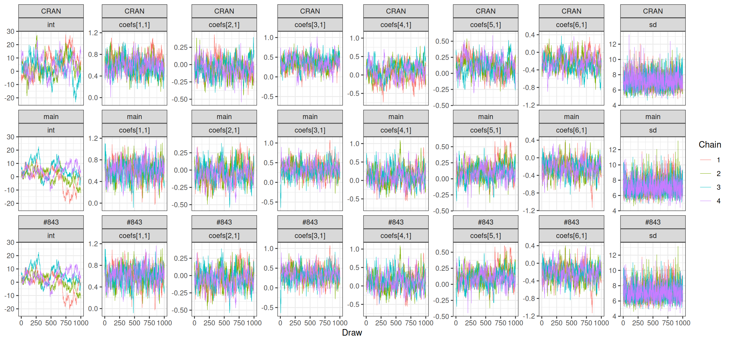
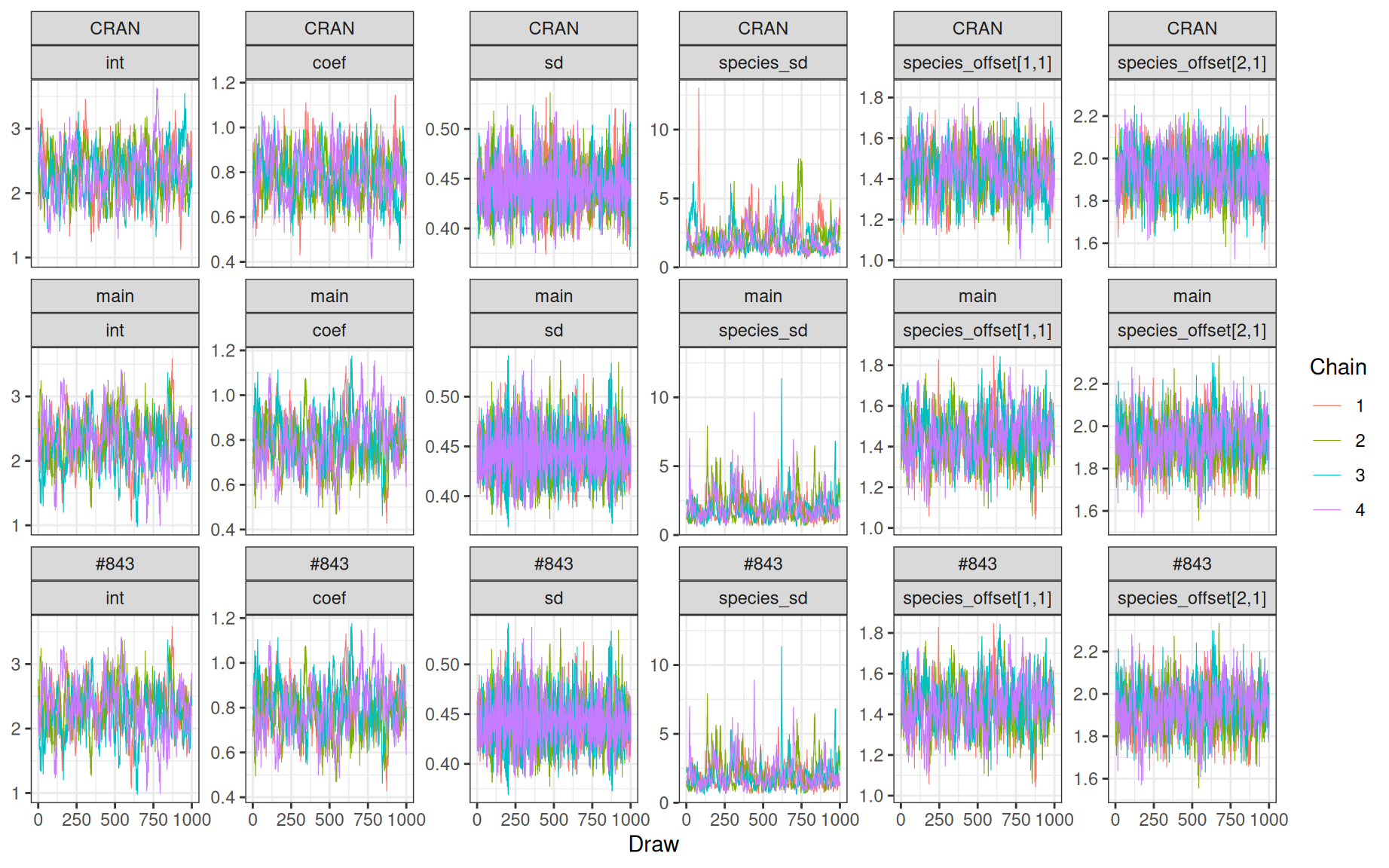
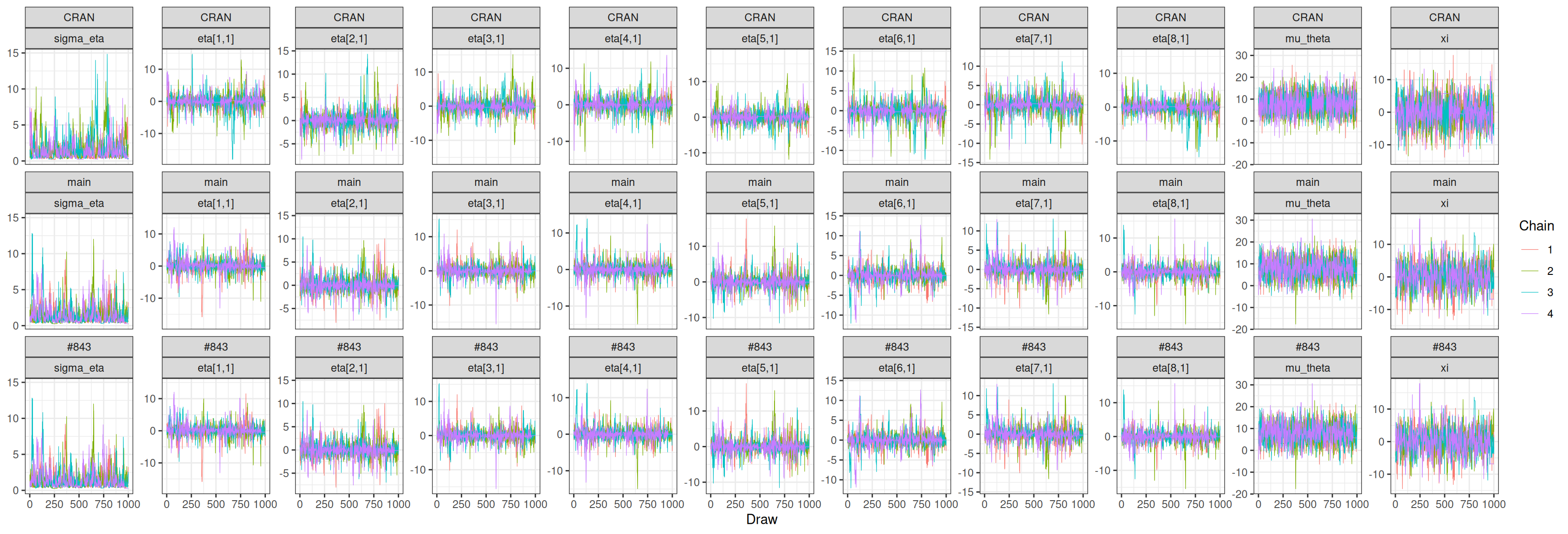
Every draw of each chain from session 1’s second mcmc() call on each model, numbered from the end of warmup, with a row of panels for each version.

# every draw of every run, one row per draw and parameter
draws <- lapply(seq_len(nrow(runs)), function(i) {
  model_draws <- runs$results[[i]]$mcmc_draws
  lapply(names(model_draws), function(model_name) {
    posterior::as_draws_df(model_draws[[model_name]]) |>
      as.data.frame() |>
      pivot_longer(
        -c(.chain, .iteration, .draw),
        names_to = "variable",
        values_to = "value"
      ) |>
      mutate(
        session = runs$session[i],
        version = runs$version[i],
        model = model_name
      )
  }) |>
    bind_rows()
}) |>
  bind_rows()

gg_trace <- function(name) {
  model_draws <- draws |>
    filter(session == 1, model == name) |>
    mutate(variable = factor(variable, levels = unique(variable)))
  # each parameter's panels share its range across the versions, so they can
  # be compared down a column
  parameter_ranges <- model_draws |>
    group_by(variable) |>
    reframe(value = range(value)) |>
    crossing(version = unique(model_draws$version)) |>
    mutate(.iteration = 1L)
  ggplot(model_draws, aes(x = .iteration, y = value, colour = factor(.chain))) +
    geom_line(linewidth = 0.2) +
    geom_blank(
      data = parameter_ranges,
      aes(x = .iteration, y = value),
      inherit.aes = FALSE
    ) +
    facet_wrap(
      vars(version, variable),
      ncol = n_distinct(model_draws$variable),
      scales = "free_y"
    ) +
    labs(x = "Draw", y = NULL, colour = "Chain")
}

linear

gg_trace("linear")

multiple_linear

gg_trace("multiple_linear")

hierarchical_linear

gg_trace("hierarchical_linear")

eight_schools

gg_trace("eight_schools")

Posterior densities

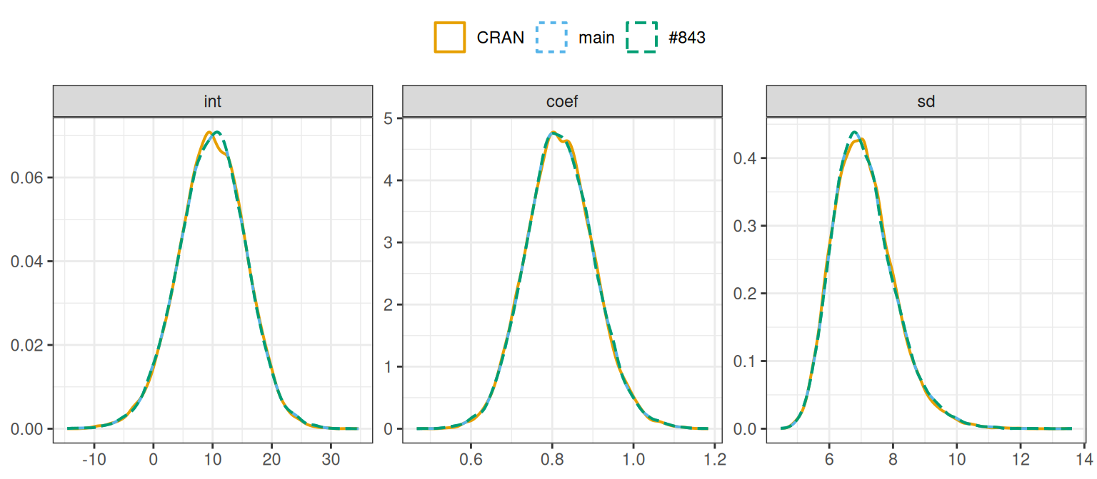
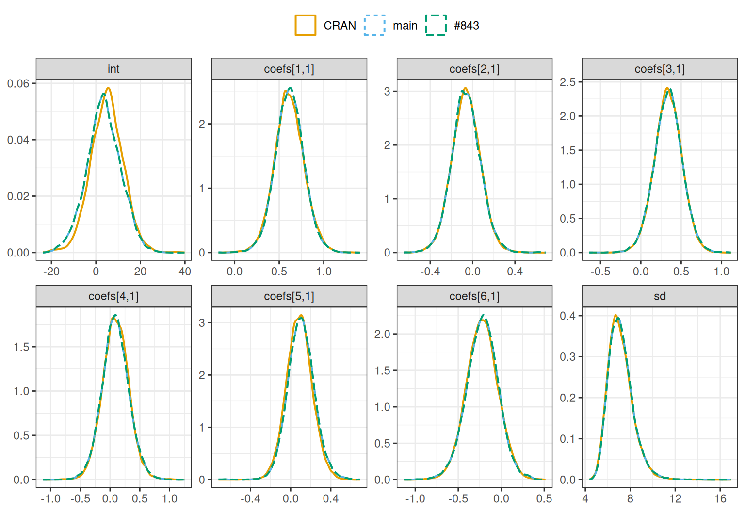
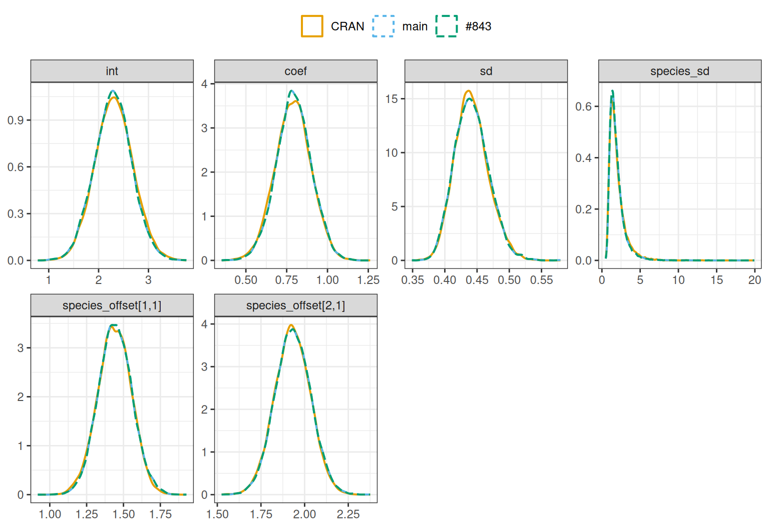
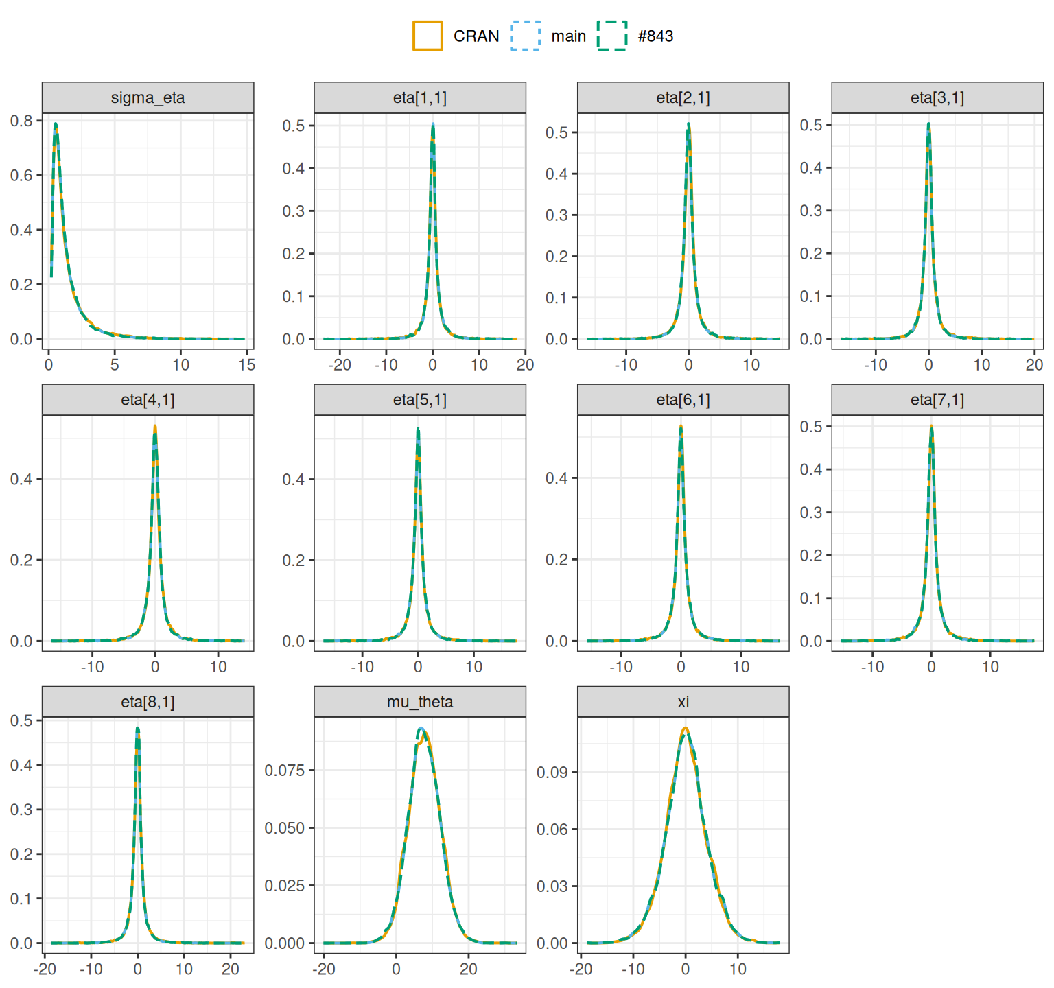
Every draw of every chain, from each session’s second mcmc() call, pooled over sessions, with every version’s density overlaid in one panel per parameter. Where two versions’ draws are identical, their lines lie on top of each other.

# every version's density in one panel per parameter, each with its own line
# type as well as colour, so a line drawn on top of an identical one still shows
gg_densities <- function(name) {
  draws |>
    filter(model == name) |>
    mutate(variable = factor(variable, levels = unique(variable))) |>
    ggplot(aes(x = value, colour = version, linetype = version)) +
    geom_density(linewidth = 0.7) +
    scale_colour_manual(values = version_colours) +
    facet_wrap(~variable, scales = "free", ncol = 4) +
    labs(x = NULL, y = NULL, colour = NULL, linetype = NULL) +
    theme(legend.position = "top")
}

densities_height <- function(name) {
  1.5 + 2 * ceiling(parameter_count(name) / 4)
}

linear

gg_densities("linear")

multiple_linear

gg_densities("multiple_linear")

hierarchical_linear

gg_densities("hierarchical_linear")

eight_schools

gg_densities("eight_schools")

Do the chains converge?

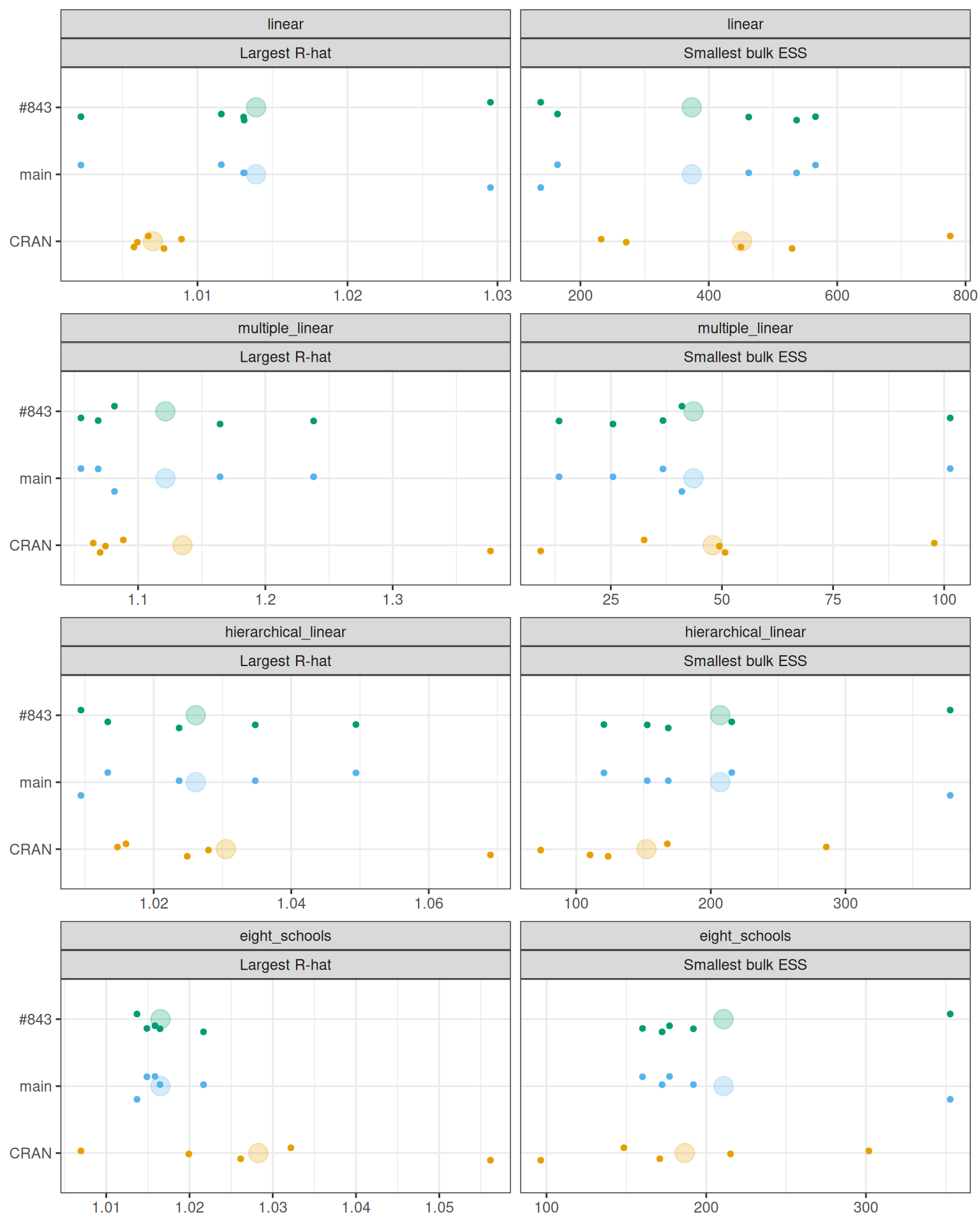
For each session’s second mcmc() call, the largest rank-normalised split-\(\hat{R}\) and the smallest bulk ESS over each model’s parameters (Vehtari et al. 2021).

convergence <- posterior |>
  group_by(session, version, model) |>
  summarise(
    largest_rhat = max(rhat),
    smallest_ess_bulk = min(ess_bulk),
    .groups = "drop"
  )

convergence_means <- convergence |>
  group_by(model, version) |>
  summarise(
    largest_rhat = mean(largest_rhat),
    smallest_ess_bulk = mean(smallest_ess_bulk),
    .groups = "drop"
  )

# one row per session, model, version and measure, for one panel per measure
convergence_measures <- c(
  largest_rhat = "Largest R-hat",
  smallest_ess_bulk = "Smallest bulk ESS"
)
longer_convergence <- function(data) {
  data |>
    pivot_longer(
      all_of(names(convergence_measures)),
      names_to = "measure",
      values_to = "value"
    ) |>
    mutate(
      measure = factor(
        convergence_measures[measure],
        levels = convergence_measures
      )
    )
}

# the model whose mean largest R-hat is largest, on any version
rhat_by_model <- convergence_means |>
  group_by(model) |>
  summarise(largest_rhat = max(largest_rhat))
worst_model <- as.character(rhat_by_model$model[which.max(rhat_by_model$largest_rhat)])
worst_rhat <- filter(convergence_means, model == worst_model)
other_models_rhat <- max(rhat_by_model$largest_rhat[rhat_by_model$model != worst_model])

ggplot(
  longer_convergence(convergence),
  aes(x = value, y = version, colour = version)
) +
  geom_point(
    data = longer_convergence(convergence_means),
    size = 5,
    alpha = 0.25
  ) +
  geom_point(position = jitter, size = 1.2) +
  version_scale +
  facet_wrap(vars(model, measure), ncol = 2, scales = "free_x") +
  labs(x = NULL, y = NULL)

Each small dot is one session’s second call. The large faint dot behind them is their mean.

From the draws kept by benchmark.R’s mcmc-draws section.

Averaged over sessions, the largest R-hat is highest on multiple_linear: CRAN 1.13, main 1.12, #843 1.12. On every other model it is at most 1.03, on every version.

Table: every session

dt_table(convergence)

How it was measured

provenance |>
  distinct(version, greta_version, greta_sha, tensorflow_version, tfp_version, r_version) |>
  arrange(version) |>
  mutate(
    installed_from = versions[as.character(version)],
    # pak records a CRAN install's version in place of a commit, so only a
    # GitHub install gets a link to its commit
    installed_from = ifelse(
      grepl("^[0-9a-f]{40}$", greta_sha),
      paste0(
        "[",
        sub("@.*", "", installed_from),
        "@",
        substr(greta_sha, 1, 8),
        "](https://github.com/greta-dev/greta/commit/",
        greta_sha,
        ")"
      ),
      installed_from
    )
  ) |>
  select(
    version,
    `installed from` = installed_from,
    greta = greta_version,
    TensorFlow = tensorflow_version,
    TFP = tfp_version,
    R = r_version
  ) |>
  knitr::kable()

version	installed from	greta	TensorFlow	TFP	R
CRAN	greta@0.6.0	0.6.0	2.15.1	0.23.0	4.6.1
main	greta-dev/greta@179021a8	0.6.0.9000	2.21.0	0.25.0	4.6.1
#843	greta-dev/greta@94ef91b9	0.6.0.9000	2.21.0	0.25.0	4.6.1

python_stacks <- provenance |>
  distinct(version, tensorflow_version, tfp_version) |>
  group_by(tensorflow_version, tfp_version) |>
  summarise(
    versions = paste_and(as.character(sort(version))),
    .groups = "drop"
  )
python_stack_text <- paste0(
  python_stacks$versions,
  " ran on TensorFlow ",
  python_stacks$tensorflow_version,
  " and TensorFlow Probability ",
  python_stacks$tfp_version,
  collapse = "; "
)

sampler_iterations_values <- sampler_iterations_per_draw |>
  group_by(version) |>
  summarise(values = paste(sort(unique(value)), collapse = " or "))

The versions are pinned to these commits in run.R’s run-versions section. CRAN ran on TensorFlow 2.15.1 and TensorFlow Probability 0.23.0; main and #843 ran on TensorFlow 2.21.0 and TensorFlow Probability 0.25.0.

Each version ran in 5 sessions, on Darwin 25.5.0 arm64 with 8 cores. In each session, run.R’s run-sessions section ran benchmark.R once per version, each in a fresh R session, with the versions in a new random order. Each session has a seed of its own, set in benchmark.R’s benchmark-setup section, and the same settings, in its benchmark-settings section.

Table: the order of each session

runs |>
  select(session, position, version) |>
  arrange(session, position) |>
  dt_table()

Every call is timed with {bench}’s mark() and saved as mark() made it, so summary() and autoplot() work on it. Under each timing, one table is bench’s summary() of every mark, with the mean and longest of its calls added, and the other has every call.

The same mcmc() arguments are the same work only if each version’s sampler runs the same number of iterations for each draw it keeps. benchmark.R’s benchmark-sampler-iterations section counts them, and in every session they were CRAN 2, main 2, #843 2.

Table: sampler iterations per kept draw, in every session

sampler_iterations_per_draw |>
  select(session, version, sampler_iterations_per_draw = value) |>
  dt_table()

Two scripts made every result here: benchmark.R is what each version runs, and run.R runs it for each version in each session. Both in full:

# Runs benchmark.R against CRAN (greta 0.6.0), main and greta#843, in a fresh R
# session per version, in five sessions:
#
#   Rscript --quiet --vanilla posts/2026-10-05-retracing-i546/run.R
#
# Each session writes results/session-<n>.rds, and sessions already there are
# skipped, so a rerun after a crash carries on. Each `# ---- label ----` line
# starts a section that index.qmd shows by that label.

# ---- run-versions ----
versions <- c(
  CRAN = "greta@0.6.0",
  main = "greta-dev/greta@179021a818cd7282896c42b03814a53556c1d98d",
  `#843` = "greta-dev/greta@94ef91b919300d33474aa3273cbb1f49cb989373"
)
n_sessions <- 5
post_dir <- here::here("posts", "2026-10-05-retracing-i546")

# ---- run-sessions ----
dir.create(file.path(post_dir, "results"), showWarnings = FALSE)

for (session in seq_len(n_sessions)) {
  session_file <- file.path(
    post_dir,
    "results",
    sprintf("session-%d.rds", session)
  )
  if (file.exists(session_file)) {
    next
  }

  # a fresh order each session, so no version is always measured first or last
  order <- sample(names(versions))

  # cross::run_versions() installs each version into a library of its own and
  # evaluates the expression in a fresh R session against it. That session
  # cannot see this one's variables, so the script's path and the session
  # number reach it as environment variables: args_callr is passed on to
  # callr::r(), whose `env` sets variables for the child process (see ?callr::r
  # and ?callr::rcmd_safe_env, whose defaults are kept).
  measured <- cross::run_versions(
    source(Sys.getenv("GRETA_BENCH_SCRIPT"), local = TRUE)$value,
    pkgs = unname(versions[order]),
    args_callr = list(
      env = c(
        callr::rcmd_safe_env(),
        GRETA_BENCH_SCRIPT = file.path(post_dir, "benchmark.R"),
        GRETA_BENCH_SESSION = session
      )
    )
  )

  saveRDS(
    list(
      session = session,
      versions = versions,
      order = order,
      results = setNames(measured$result, order)
    ),
    session_file,
    compress = "xz"
  )
}

# What each version of greta runs, in a fresh R session of its own: run.R
# sources it once per version per session, and keeps the list it ends with.
# Each `# ---- label ----` line starts a section that index.qmd shows by that
# label.
#
# Run it alone to try it against whichever greta is installed:
#
#   Rscript --quiet --vanilla posts/2026-10-05-retracing-i546/benchmark.R

# ---- benchmark-setup ----
library(greta)
library(bench)
session <- as.integer(Sys.getenv("GRETA_BENCH_SESSION", "1"))
session_seed <- 2026 - 10 - 5 + session

# ---- benchmark-settings ----
# warmup and n_samples are mcmc()'s arguments, so they count draws; the
# *_calls settings count timed calls
bench_settings <- list(
  warmup = 1000,
  n_samples = 1000,
  chains = 4,
  n_cores = 4,
  build_calls = 5,
  opt_calls = 5,
  hessian_calls = 3,
  mcmc_calls = 2
)

# ---- model-linear ----
build_linear <- function() {
  int <- normal(0, 10)
  coef <- normal(0, 10)
  sd <- cauchy(0, 3, truncation = c(0, Inf))
  mu <- int + coef * attitude$complaints
  distribution(attitude$rating) <- normal(mu, sd)
  model(int, coef, sd)
}

# ---- model-multiple-linear ----
build_multiple_linear <- function() {
  design <- as.matrix(attitude[, 2:7])
  int <- normal(0, 10)
  coefs <- normal(0, 10, dim = ncol(design))
  sd <- cauchy(0, 3, truncation = c(0, Inf))
  mu <- int + design %*% coefs
  distribution(attitude$rating) <- normal(mu, sd)
  model(int, coefs, sd)
}

# ---- model-hierarchical-linear ----
build_hierarchical_linear <- function() {
  int <- normal(0, 10)
  coef <- normal(0, 10)
  sd <- cauchy(0, 3, truncation = c(0, Inf))
  species_sd <- lognormal(0, 1)
  species_offset <- normal(0, species_sd, dim = 2)
  species_effect <- rbind(0, species_offset)
  species_id <- as.numeric(iris$Species)
  mu <- int + coef * iris$Sepal.Width + species_effect[species_id]
  distribution(iris$Sepal.Length) <- normal(mu, sd)
  model(int, coef, sd, species_sd, species_offset)
}

# ---- model-eight-schools ----
build_eight_schools <- function() {
  y <- c(28, 8, -3, 7, -1, 1, 18, 12)
  sigma_y <- c(15, 10, 16, 11, 9, 11, 10, 18)
  sigma_eta <- inverse_gamma(1, 1)
  eta <- normal(0, sigma_eta, dim = 8)
  mu_theta <- normal(0, 100)
  xi <- normal(0, 5)
  theta <- mu_theta + xi * eta
  distribution(y) <- normal(theta, sigma_y)
  model(sigma_eta, eta, mu_theta, xi)
}

# ---- model-hessian ----
# The model greta#546 reported: twenty separate scalar parameters, each needing
# its own hessian. Its data are simulated once, with a seed of their own, so
# building the model leaves the session's random numbers alone.
hessian_y <- withr::with_seed(2026 - 09 - 29, rnorm(20))

build_hessian <- function() {
  y <- hessian_y
  target_names <- paste0("b", 1:20)
  for (name in target_names) {
    assign(name, variable())
  }
  distribution(y) <- normal(do.call(c, mget(target_names)), 1)
  # model() names its targets from the expressions it is given, so the call is
  # built from the names: this is model(b1, b2, ..., b20)
  eval(as.call(c(quote(model), lapply(target_names, as.name))))
}

# ---- benchmark-helpers ----
# TensorFlow logs its retracing warning through Python's logging, which R does
# not see, so point that logger at stderr and capture stderr
count_retracing_warnings <- function(expr) {
  captured <- reticulate::py_capture_output(
    {
      reticulate::py_run_string(paste(
        "import sys",
        "from tensorflow.python.platform import tf_logging",
        "for _h in tf_logging.get_logger().handlers: _h.stream = sys.stderr",
        sep = "\n"
      ))
      force(expr)
    },
    type = "stderr"
  )
  sum(grepl("triggered tf.function retracing", strsplit(captured, "\n")[[1]]))
}

# how many times each of a model's TensorFlow functions has been traced
count_traces <- function(model_name, model, draws) {
  traces <- function(tf_function) {
    tryCatch(
      as.integer(tf_function$experimental_get_tracing_count()),
      error = function(e) NA_integer_
    )
  }
  sampler <- attr(draws, "model_info")$samplers[[1]]
  data.frame(
    model = model_name,
    log_prob_traces = traces(model$dag$tf_log_prob_function),
    trace_values_traces = traces(model$dag$tf_trace_values_batch),
    sampler_traces = traces(sampler$tf_evaluate_sample_batch)
  )
}

# ---- benchmark-sampler-iterations ----
# A random walk on a target far wider than its steps accepts every proposal, so
# the variance between kept draws over one step's variance counts the sampler
# iterations between them. It is also the session's first mcmc() call, so
# TensorFlow's start-up costs fall here rather than on the first model.
step_sd <- 0.1
x <- normal(0, 1e6)
walk <- mcmc(
  model(x),
  sampler = rwmh(epsilon = step_sd, diag_sd = 1),
  warmup = 0,
  n_samples = 4000,
  thin = 1,
  chains = 1,
  initial_values = initials(x = 0),
  verbose = FALSE
)
sampler_iterations_per_draw <- round(
  var(diff(as.vector(walk[[1]]))) / step_sd^2
)

# ---- bench-build-linear ----
# mark()'s `iterations` is how many times it calls the expression
build_linear
bench_build_linear <- mark(
  build_linear(),
  iterations = bench_settings$build_calls,
  check = FALSE,
  memory = FALSE,
  filter_gc = FALSE
)

# ---- bench-build-multiple-linear ----
build_multiple_linear
bench_build_multiple_linear <- mark(
  build_multiple_linear(),
  iterations = bench_settings$build_calls,
  check = FALSE,
  memory = FALSE,
  filter_gc = FALSE
)

# ---- bench-build-hierarchical-linear ----
build_hierarchical_linear
bench_build_hierarchical_linear <- mark(
  build_hierarchical_linear(),
  iterations = bench_settings$build_calls,
  check = FALSE,
  memory = FALSE,
  filter_gc = FALSE
)

# ---- bench-build-eight-schools ----
build_eight_schools
bench_build_eight_schools <- mark(
  build_eight_schools(),
  iterations = bench_settings$build_calls,
  check = FALSE,
  memory = FALSE,
  filter_gc = FALSE
)

# ---- bench-opt ----
# opt() draws its starting values from R's random numbers, so each model's
# calls start from the same seed
# ---- bench-opt-linear ----
build_linear
linear_for_opt <- build_linear()
set.seed(session_seed)
bench_opt_linear <- mark(
  opt(linear_for_opt),
  iterations = bench_settings$opt_calls,
  check = FALSE,
  memory = FALSE,
  filter_gc = FALSE
)

# ---- bench-opt-multiple-linear ----
build_multiple_linear
multiple_linear_for_opt <- build_multiple_linear()
set.seed(session_seed)
bench_opt_multiple_linear <- mark(
  opt(multiple_linear_for_opt),
  iterations = bench_settings$opt_calls,
  check = FALSE,
  memory = FALSE,
  filter_gc = FALSE
)

# ---- bench-opt-hierarchical-linear ----
build_hierarchical_linear
hierarchical_linear_for_opt <- build_hierarchical_linear()
set.seed(session_seed)
bench_opt_hierarchical_linear <- mark(
  opt(hierarchical_linear_for_opt),
  iterations = bench_settings$opt_calls,
  check = FALSE,
  memory = FALSE,
  filter_gc = FALSE
)

# ---- bench-opt-eight-schools ----
build_eight_schools
eight_schools_for_opt <- build_eight_schools()
set.seed(session_seed)
bench_opt_eight_schools <- mark(
  opt(eight_schools_for_opt),
  iterations = bench_settings$opt_calls,
  check = FALSE,
  memory = FALSE,
  filter_gc = FALSE
)

# ---- bench-hessian ----
build_hessian
hessian_for_opt <- build_hessian()
set.seed(session_seed)
hessian_retracing_warnings <- count_retracing_warnings(
  bench_hessian <- mark(
    opt(hessian_for_opt, hessian = TRUE),
    iterations = bench_settings$hessian_calls,
    check = FALSE,
    memory = FALSE,
    filter_gc = FALSE
  )
)

# ---- bench-mcmc ----
# Both of a model's calls are on the same model: the first traces its
# TensorFlow functions and the second reuses them. Each `draws_` object keeps
# the second call's draws.

# ---- bench-mcmc-linear ----
build_linear
linear_for_mcmc <- build_linear()
set.seed(session_seed)
mcmc_retracing_warnings_linear <- count_retracing_warnings(
  bench_mcmc_linear <- mark(
    draws_linear <- mcmc(
      linear_for_mcmc,
      warmup = bench_settings$warmup,
      n_samples = bench_settings$n_samples,
      chains = bench_settings$chains,
      n_cores = bench_settings$n_cores,
      verbose = FALSE
    ),
    iterations = bench_settings$mcmc_calls,
    check = FALSE,
    memory = FALSE,
    filter_gc = FALSE
  )
)

# ---- bench-mcmc-multiple-linear ----
build_multiple_linear
multiple_linear_for_mcmc <- build_multiple_linear()
set.seed(session_seed)
mcmc_retracing_warnings_multiple_linear <- count_retracing_warnings(
  bench_mcmc_multiple_linear <- mark(
    draws_multiple_linear <- mcmc(
      multiple_linear_for_mcmc,
      warmup = bench_settings$warmup,
      n_samples = bench_settings$n_samples,
      chains = bench_settings$chains,
      n_cores = bench_settings$n_cores,
      verbose = FALSE
    ),
    iterations = bench_settings$mcmc_calls,
    check = FALSE,
    memory = FALSE,
    filter_gc = FALSE
  )
)

# ---- bench-mcmc-hierarchical-linear ----
build_hierarchical_linear
hierarchical_linear_for_mcmc <- build_hierarchical_linear()
set.seed(session_seed)
mcmc_retracing_warnings_hierarchical_linear <- count_retracing_warnings(
  bench_mcmc_hierarchical_linear <- mark(
    draws_hierarchical_linear <- mcmc(
      hierarchical_linear_for_mcmc,
      warmup = bench_settings$warmup,
      n_samples = bench_settings$n_samples,
      chains = bench_settings$chains,
      n_cores = bench_settings$n_cores,
      verbose = FALSE
    ),
    iterations = bench_settings$mcmc_calls,
    check = FALSE,
    memory = FALSE,
    filter_gc = FALSE
  )
)

# ---- bench-mcmc-eight-schools ----
build_eight_schools
eight_schools_for_mcmc <- build_eight_schools()
set.seed(session_seed)
mcmc_retracing_warnings_eight_schools <- count_retracing_warnings(
  bench_mcmc_eight_schools <- mark(
    draws_eight_schools <- mcmc(
      eight_schools_for_mcmc,
      warmup = bench_settings$warmup,
      n_samples = bench_settings$n_samples,
      chains = bench_settings$chains,
      n_cores = bench_settings$n_cores,
      verbose = FALSE
    ),
    iterations = bench_settings$mcmc_calls,
    check = FALSE,
    memory = FALSE,
    filter_gc = FALSE
  )
)

# ---- mcmc-tracing ----
# each model's trace counts after both calls, and the retracing warnings
# TensorFlow logged during them
mcmc_tracing <- rbind(
  count_traces("linear", linear_for_mcmc, draws_linear),
  count_traces(
    "multiple_linear",
    multiple_linear_for_mcmc,
    draws_multiple_linear
  ),
  count_traces(
    "hierarchical_linear",
    hierarchical_linear_for_mcmc,
    draws_hierarchical_linear
  ),
  count_traces("eight_schools", eight_schools_for_mcmc, draws_eight_schools)
)
mcmc_tracing$retracing_warnings <- c(
  mcmc_retracing_warnings_linear,
  mcmc_retracing_warnings_multiple_linear,
  mcmc_retracing_warnings_hierarchical_linear,
  mcmc_retracing_warnings_eight_schools
)

# ---- mcmc-draws ----
# Every draw of every chain from each model's second call. A posterior draws
# array holds just the draws: the greta_mcmc_list mcmc() returns carries the
# model and its TensorFlow objects, which cannot be saved.
mcmc_draws <- list(
  linear = posterior::as_draws_array(draws_linear),
  multiple_linear = posterior::as_draws_array(draws_multiple_linear),
  hierarchical_linear = posterior::as_draws_array(draws_hierarchical_linear),
  eight_schools = posterior::as_draws_array(draws_eight_schools)
)

# ---- benchmark-provenance ----
session_info <- sessioninfo::session_info()
# greta_sitrep() reports through messages, so capture those
greta_sitrep_report <- utils::capture.output(greta_sitrep(), type = "message")

greta_sha <- packageDescription("greta")$RemoteSha
provenance <- data.frame(
  greta_version = as.character(packageVersion("greta")),
  greta_sha = if (is.null(greta_sha)) NA_character_ else greta_sha,
  r_version = paste(R.version$major, R.version$minor, sep = "."),
  tensorflow_version = tensorflow::tf$version$VERSION,
  tfp_version = reticulate::import("tensorflow_probability")$`__version__`,
  machine = paste(
    Sys.info()[c("sysname", "release", "machine")],
    collapse = " "
  ),
  cores = parallel::detectCores()
)

# ---- benchmark-results ----
# the value source() returns to run.R: every bench_mark object as mark() made
# it, and the summaries beside them
list(
  session_seed = session_seed,
  bench_settings = bench_settings,
  provenance = provenance,
  session_info = session_info,
  greta_sitrep_report = greta_sitrep_report,
  sampler_iterations_per_draw = sampler_iterations_per_draw,
  build = list(
    linear = bench_build_linear,
    multiple_linear = bench_build_multiple_linear,
    hierarchical_linear = bench_build_hierarchical_linear,
    eight_schools = bench_build_eight_schools
  ),
  opt = list(
    linear = bench_opt_linear,
    multiple_linear = bench_opt_multiple_linear,
    hierarchical_linear = bench_opt_hierarchical_linear,
    eight_schools = bench_opt_eight_schools
  ),
  hessian = bench_hessian,
  hessian_retracing_warnings = hessian_retracing_warnings,
  mcmc = list(
    linear = bench_mcmc_linear,
    multiple_linear = bench_mcmc_multiple_linear,
    hierarchical_linear = bench_mcmc_hierarchical_linear,
    eight_schools = bench_mcmc_eight_schools
  ),
  mcmc_tracing = mcmc_tracing,
  mcmc_draws = mcmc_draws
)

The models

Four models are from greta’s inst/examples/; the hessian model is the one greta#546 reported. Normal and log-normal distributions are written with their mean and standard deviation, as greta’s normal() and lognormal() take them; \(\text{Cauchy}^{+}\) is a Cauchy truncated to positive values.

linear

A regression of each department’s rating in attitude on its number of complaints. 3 parameters.

\[ \begin{aligned} \text{rating}_i &\sim \text{Normal}(\mu_i, \sigma), \quad i = 1, \dots, 30 \\ \mu_i &= \alpha + \beta \, \text{complaints}_i \\ \alpha, \beta &\sim \text{Normal}(0, 10) \\ \sigma &\sim \text{Cauchy}^{+}(0, 3) \end{aligned} \]

build_linear <- function() {
  int <- normal(0, 10)
  coef <- normal(0, 10)
  sd <- cauchy(0, 3, truncation = c(0, Inf))
  mu <- int + coef * attitude$complaints
  distribution(attitude$rating) <- normal(mu, sd)
  model(int, coef, sd)
}

multiple_linear

The same rating on all six of attitude’s other columns, \(X\), through a matrix multiply. 8 parameters.

\[ \begin{aligned} \text{rating}_i &\sim \text{Normal}(\mu_i, \sigma), \quad i = 1, \dots, 30 \\ \mu_i &= \alpha + \sum_{j = 1}^{6} X_{ij} \, \beta_j \\ \alpha, \beta_j &\sim \text{Normal}(0, 10) \\ \sigma &\sim \text{Cauchy}^{+}(0, 3) \end{aligned} \]

build_multiple_linear <- function() {
  design <- as.matrix(attitude[, 2:7])
  int <- normal(0, 10)
  coefs <- normal(0, 10, dim = ncol(design))
  sd <- cauchy(0, 3, truncation = c(0, Inf))
  mu <- int + design %*% coefs
  distribution(attitude$rating) <- normal(mu, sd)
  model(int, coefs, sd)
}

hierarchical_linear

Sepal length on sepal width in iris, with an offset for each species, \(s[i]\) being flower \(i\)’s. Setosa’s offset is zero and the other two share a scale, \(\tau\). 6 parameters.

\[ \begin{aligned} \text{Sepal.Length}_i &\sim \text{Normal}(\mu_i, \sigma), \quad i = 1, \dots, 150 \\ \mu_i &= \alpha + \beta \, \text{Sepal.Width}_i + \gamma_{s[i]} \\ \gamma_1 &= 0, \qquad \gamma_2, \gamma_3 \sim \text{Normal}(0, \tau) \\ \tau &\sim \text{LogNormal}(0, 1) \\ \alpha, \beta &\sim \text{Normal}(0, 10) \\ \sigma &\sim \text{Cauchy}^{+}(0, 3) \end{aligned} \]

build_hierarchical_linear <- function() {
  int <- normal(0, 10)
  coef <- normal(0, 10)
  sd <- cauchy(0, 3, truncation = c(0, Inf))
  species_sd <- lognormal(0, 1)
  species_offset <- normal(0, species_sd, dim = 2)
  species_effect <- rbind(0, species_offset)
  species_id <- as.numeric(iris$Species)
  mu <- int + coef * iris$Sepal.Width + species_effect[species_id]
  distribution(iris$Sepal.Length) <- normal(mu, sd)
  model(int, coef, sd, species_sd, species_offset)
}

eight_schools

The effect of coaching in eight schools, \(y_j\), each measured with a known standard error, \(\sigma_j\). The scale of the school effects, \(\sigma_\eta\), is itself a parameter, which makes the posterior a funnel. 11 parameters.

\[ \begin{aligned} y_j &\sim \text{Normal}(\theta_j, \sigma_j), \quad j = 1, \dots, 8 \\ \theta_j &= \mu + \xi \, \eta_j \\ \eta_j &\sim \text{Normal}(0, \sigma_\eta) \\ \sigma_\eta &\sim \text{InverseGamma}(1, 1) \\ \mu &\sim \text{Normal}(0, 100) \\ \xi &\sim \text{Normal}(0, 5) \end{aligned} \]

build_eight_schools <- function() {
  y <- c(28, 8, -3, 7, -1, 1, 18, 12)
  sigma_y <- c(15, 10, 16, 11, 9, 11, 10, 18)
  sigma_eta <- inverse_gamma(1, 1)
  eta <- normal(0, sigma_eta, dim = 8)
  mu_theta <- normal(0, 100)
  xi <- normal(0, 5)
  theta <- mu_theta + xi * eta
  distribution(y) <- normal(theta, sigma_y)
  model(sigma_eta, eta, mu_theta, xi)
}

hessian model

Used only for opt(hessian = TRUE): twenty simulated observations \(y_k\), each with its own mean \(b_k\), so each call takes twenty hessians. greta’s variable() gives \(b_k\) a flat prior, so it has no distribution line.

\[ y_k \sim \text{Normal}(b_k, 1), \quad k = 1, \dots, 20 \]

# The model greta#546 reported: twenty separate scalar parameters, each needing
# its own hessian. Its data are simulated once, with a seed of their own, so
# building the model leaves the session's random numbers alone.
hessian_y <- withr::with_seed(2026 - 09 - 29, rnorm(20))

build_hessian <- function() {
  y <- hessian_y
  target_names <- paste0("b", 1:20)
  for (name in target_names) {
    assign(name, variable())
  }
  distribution(y) <- normal(do.call(c, mget(target_names)), 1)
  # model() names its targets from the expressions it is given, so the call is
  # built from the names: this is model(b1, b2, ..., b20)
  eval(as.call(c(quote(model), lapply(target_names, as.name))))
}

Session details

What each version reported about itself in session 1, from benchmark.R’s benchmark-provenance section.

session_one <- runs |>
  filter(session == 1) |>
  arrange(version)

# a saved session_info() prints with sessioninfo's print method, which is
# registered only once its namespace is loaded
invisible(loadNamespace("sessioninfo"))

CRAN

greta_sitrep()

writeLines(session_one$results[[which(session_one$version == "CRAN")]]$greta_sitrep_report)

ℹ checking if python available
✔ python (v3.11) available

ℹ checking if TensorFlow available
✔ TensorFlow (v2.15.1) available

ℹ checking if TensorFlow Probability available
✔ TensorFlow Probability (v0.23.0) available

ℹ greta conda environment: not used (managed (uv) environment active)
• backend: "managed (uv) environment"
• selected via: default
✔ offline-ready: uv cache present, offline mode will engage
ℹ All dependencies available; greta is ready to use!

sessioninfo::session_info()

session_one$results[[which(session_one$version == "CRAN")]]$session_info

─ Session info ───────────────────────────────────────────────────────────────
 setting  value
 version  R version 4.6.1 (2026-06-24)
 os       macOS Tahoe 26.5.2
 system   aarch64, darwin23
 ui       X11
 language (EN)
 collate  en_AU.UTF-8
 ctype    en_AU.UTF-8
 tz       Australia/Hobart
 date     2026-10-05
 pandoc   3.10 @ /opt/homebrew/bin/pandoc
 quarto   1.9.36 @ /usr/local/bin/quarto

─ Packages ───────────────────────────────────────────────────────────────────
 package        * version  date (UTC) lib source
 abind            1.4-8    2024-09-12 [1] CRAN (R 4.6.0)
 backports        1.5.1    2026-04-03 [1] CRAN (R 4.6.0)
 base64enc        0.1-6    2026-02-02 [1] CRAN (R 4.6.0)
 bench          * 1.1.4    2025-01-16 [3] CRAN (R 4.6.0)
 callr            3.8.0    2026-06-05 [1] CRAN (R 4.6.0)
 checkmate        2.3.4    2026-02-03 [2] CRAN (R 4.6.0)
 cli              3.6.6    2026-04-09 [1] CRAN (R 4.6.0)
 coda             0.19-4.1 2024-01-31 [1] CRAN (R 4.6.0)
 codetools        0.2-20   2024-03-31 [3] CRAN (R 4.6.1)
 crayon           1.5.3    2024-06-20 [1] CRAN (R 4.6.0)
 digest           0.6.39   2025-11-19 [1] CRAN (R 4.6.0)
 distributional   0.9.0    2026-09-08 [2] CRAN (R 4.6.1)
 future           1.76.0   2026-09-24 [1] CRAN (R 4.6.1)
 generics         0.1.4    2025-05-09 [2] CRAN (R 4.6.0)
 globals          0.19.1   2026-03-13 [1] CRAN (R 4.6.0)
 glue             1.8.1    2026-04-17 [1] CRAN (R 4.6.0)
 greta          * 0.6.0    2026-07-20 [1] CRAN (R 4.6.1)
 hms              1.1.4    2025-10-17 [1] CRAN (R 4.6.0)
 jsonlite         2.0.0    2025-03-27 [1] CRAN (R 4.6.0)
 lattice          0.23-1   2026-08-12 [3] CRAN (R 4.6.1)
 lifecycle        1.0.5    2026-01-08 [1] CRAN (R 4.6.0)
 listenv          1.0.0    2026-06-22 [1] CRAN (R 4.6.1)
 magrittr         2.0.5    2026-04-04 [1] CRAN (R 4.6.0)
 Matrix           1.7-6    2026-07-25 [3] CRAN (R 4.6.1)
 parallelly       1.48.0   2026-06-29 [1] CRAN (R 4.6.1)
 pillar           1.11.1   2025-09-17 [2] CRAN (R 4.6.0)
 pkgconfig        2.0.3    2019-09-22 [1] CRAN (R 4.6.0)
 png              0.1-9    2026-03-15 [1] CRAN (R 4.6.0)
 posterior        1.7.0    2026-04-01 [2] CRAN (R 4.6.0)
 prettyunits      1.2.0    2023-09-24 [1] CRAN (R 4.6.0)
 processx         3.9.0    2026-04-22 [1] CRAN (R 4.6.0)
 progress         1.2.3    2023-12-06 [1] CRAN (R 4.6.0)
 R6               2.6.1    2025-02-15 [1] CRAN (R 4.6.0)
 Rcpp             1.1.2    2026-07-05 [1] CRAN (R 4.6.1)
 reticulate       1.47.0   2026-09-03 [1] CRAN (R 4.6.1)
 rlang            1.3.0    2026-07-05 [1] CRAN (R 4.6.1)
 sessioninfo      1.2.4    2026-06-04 [3] CRAN (R 4.6.0)
 tensorA          0.36.2.1 2023-12-13 [2] CRAN (R 4.6.0)
 tensorflow       2.20.0   2025-08-22 [1] CRAN (R 4.6.0)
 tfautograph      0.3.2    2021-09-17 [1] CRAN (R 4.6.0)
 tfruns           1.5.4    2025-08-20 [1] CRAN (R 4.6.0)
 tibble           3.3.1    2026-01-11 [2] CRAN (R 4.6.0)
 vctrs            0.7.3    2026-04-11 [1] CRAN (R 4.6.0)
 whisker          0.4.1    2022-12-05 [1] CRAN (R 4.6.0)
 withr            3.0.3    2026-06-19 [1] CRAN (R 4.6.0)

 [1] /private/var/folders/cz/hrp33k3s0jlcb_gg9snlqh580000gq/T/Rtmp09vUZy/file626b3b11580e
 [2] /Users/nick_1/Library/R/arm64/4.6/library
 [3] /Library/Frameworks/R.framework/Versions/4.6/Resources/library
 * ── Packages attached to the search path.

─ Python configuration ───────────────────────────────────────────────────────
 /Users/nick_1/.cache/uv/archive-v0/UHNUTkY5VFNKpV0lCgUGo/bin/python
 /Users/nick_1/.local/share/uv/python/cpython-3.11.15-macos-aarch64-none/lib/libpython3.11.dylib
 /Users/nick_1/.cache/uv/archive-v0/UHNUTkY5VFNKpV0lCgUGo:/Users/nick_1/.cache/uv/archive-v0/UHNUTkY5VFNKpV0lCgUGo
 /Users/nick_1/.local/share/uv/python/cpython-3.11.15-macos-aarch64-none/lib/python311.zip:/Users/nick_1/.local/share/uv/python/cpython-3.11.15-macos-aarch64-none/lib/python3.11:/Users/nick_1/.local/share/uv/python/cpython-3.11.15-macos-aarch64-none/lib/python3.11/lib-dynload:/Users/nick_1/.cache/uv/archive-v0/UHNUTkY5VFNKpV0lCgUGo/lib/python3.11/site-packages
 /Users/nick_1/.cache/uv/archive-v0/UHNUTkY5VFNKpV0lCgUGo
 /Users/nick_1/.cache/uv/archive-v0/UHNUTkY5VFNKpV0lCgUGo
 /Users/nick_1/.local/share/uv/python/cpython-3.11.15-macos-aarch64-none
 /Users/nick_1/.cache/uv/archive-v0/UHNUTkY5VFNKpV0lCgUGo
 /Users/nick_1/.cache/uv/archive-v0/UHNUTkY5VFNKpV0lCgUGo/bin/activate_this.py
 /Users/nick_1/.cache/uv/archive-v0/UHNUTkY5VFNKpV0lCgUGo/bin/python
 /Users/nick_1/.local/share/uv/python/cpython-3.11.15-macos-aarch64-none/bin/python3.11
 3.11.15 (main, Mar 20 2026, 00:41:54) [Clang 22.1.1 ]
 3, 11
 64bit
 FALSE
 False
 /Users/nick_1/.cache/uv/archive-v0/UHNUTkY5VFNKpV0lCgUGo/lib/python3.11/site-packages/numpy, 1                                                                                          , 26                                                                                         , 4                                                                                          
 tensorflow
 /Users/nick_1/.cache/uv/archive-v0/UHNUTkY5VFNKpV0lCgUGo/lib/python3.11/site-packages/tensorflow
 TRUE
 /Users/nick_1/.cache/uv/archive-v0/UHNUTkY5VFNKpV0lCgUGo/bin/python
 py_require()
 TRUE

──────────────────────────────────────────────────────────────────────────────

main

greta_sitrep()

writeLines(session_one$results[[which(session_one$version == "main")]]$greta_sitrep_report)

ℹ checking if python available
✔ python (v3.12) available

ℹ checking if TensorFlow available
✔ TensorFlow (v2.21.0) available

ℹ checking if TensorFlow Probability available
✔ TensorFlow Probability (v0.25.0) available

ℹ greta conda environment: not used (managed (uv) environment active)
• backend: "managed (uv) environment"
• selected via: default
✔ offline-ready: `UV_OFFLINE`=1 is set and the uv cache is populated
ℹ All dependencies available; greta is ready to use!

sessioninfo::session_info()

session_one$results[[which(session_one$version == "main")]]$session_info

─ Session info ───────────────────────────────────────────────────────────────
 setting  value
 version  R version 4.6.1 (2026-06-24)
 os       macOS Tahoe 26.5.2
 system   aarch64, darwin23
 ui       X11
 language (EN)
 collate  en_AU.UTF-8
 ctype    en_AU.UTF-8
 tz       Australia/Hobart
 date     2026-10-05
 pandoc   3.10 @ /opt/homebrew/bin/pandoc
 quarto   1.9.36 @ /usr/local/bin/quarto

─ Packages ───────────────────────────────────────────────────────────────────
 package        * version    date (UTC) lib source
 abind            1.4-8      2024-09-12 [1] CRAN (R 4.6.0)
 backports        1.5.1      2026-04-03 [1] CRAN (R 4.6.0)
 base64enc        0.1-6      2026-02-02 [1] CRAN (R 4.6.0)
 bench          * 1.1.4      2025-01-16 [3] CRAN (R 4.6.0)
 callr            3.8.0      2026-06-05 [1] CRAN (R 4.6.0)
 checkmate        2.3.4      2026-02-03 [2] CRAN (R 4.6.0)
 cli              3.6.6      2026-04-09 [1] CRAN (R 4.6.0)
 coda             0.19-4.1   2024-01-31 [1] CRAN (R 4.6.0)
 codetools        0.2-20     2024-03-31 [3] CRAN (R 4.6.1)
 crayon           1.5.3      2024-06-20 [1] CRAN (R 4.6.0)
 digest           0.6.39     2025-11-19 [1] CRAN (R 4.6.0)
 distributional   0.9.0      2026-09-08 [2] CRAN (R 4.6.1)
 future           1.76.0     2026-09-24 [1] CRAN (R 4.6.1)
 generics         0.1.4      2025-05-09 [2] CRAN (R 4.6.0)
 globals          0.19.1     2026-03-13 [1] CRAN (R 4.6.0)
 glue             1.8.1      2026-04-17 [1] CRAN (R 4.6.0)
 greta          * 0.6.0.9000 2026-10-04 [1] Github (greta-dev/greta@179021a)
 hms              1.1.4      2025-10-17 [1] CRAN (R 4.6.0)
 jsonlite         2.0.0      2025-03-27 [1] CRAN (R 4.6.0)
 lattice          0.23-1     2026-08-12 [3] CRAN (R 4.6.1)
 lifecycle        1.0.5      2026-01-08 [1] CRAN (R 4.6.0)
 listenv          1.0.0      2026-06-22 [1] CRAN (R 4.6.1)
 magrittr         2.0.5      2026-04-04 [1] CRAN (R 4.6.0)
 Matrix           1.7-6      2026-07-25 [3] CRAN (R 4.6.1)
 parallelly       1.48.0     2026-06-29 [1] CRAN (R 4.6.1)
 pillar           1.11.1     2025-09-17 [2] CRAN (R 4.6.0)
 pkgconfig        2.0.3      2019-09-22 [1] CRAN (R 4.6.0)
 png              0.1-9      2026-03-15 [1] CRAN (R 4.6.0)
 posterior        1.7.0      2026-04-01 [2] CRAN (R 4.6.0)
 prettyunits      1.2.0      2023-09-24 [1] CRAN (R 4.6.0)
 processx         3.9.0      2026-04-22 [1] CRAN (R 4.6.0)
 progress         1.2.3      2023-12-06 [1] CRAN (R 4.6.0)
 R6               2.6.1      2025-02-15 [1] CRAN (R 4.6.0)
 Rcpp             1.1.2      2026-07-05 [1] CRAN (R 4.6.1)
 reticulate       1.47.0     2026-09-03 [1] CRAN (R 4.6.1)
 rlang            1.3.0      2026-07-05 [1] CRAN (R 4.6.1)
 sessioninfo      1.2.4      2026-06-04 [3] CRAN (R 4.6.0)
 tensorA          0.36.2.1   2023-12-13 [2] CRAN (R 4.6.0)
 tensorflow       2.20.0     2025-08-22 [1] CRAN (R 4.6.0)
 tfautograph      0.3.2      2021-09-17 [1] CRAN (R 4.6.0)
 tfruns           1.5.4      2025-08-20 [1] CRAN (R 4.6.0)
 tibble           3.3.1      2026-01-11 [2] CRAN (R 4.6.0)
 vctrs            0.7.3      2026-04-11 [1] CRAN (R 4.6.0)
 whisker          0.4.1      2022-12-05 [1] CRAN (R 4.6.0)
 withr            3.0.3      2026-06-19 [1] CRAN (R 4.6.0)

 [1] /private/var/folders/cz/hrp33k3s0jlcb_gg9snlqh580000gq/T/Rtmp09vUZy/file626b6fac1d6d
 [2] /Users/nick_1/Library/R/arm64/4.6/library
 [3] /Library/Frameworks/R.framework/Versions/4.6/Resources/library
 * ── Packages attached to the search path.

─ Python configuration ───────────────────────────────────────────────────────
 /Users/nick_1/.cache/uv/archive-v0/L7vrsM8H3lbjoC0FIwGSF/bin/python
 /Users/nick_1/.local/share/uv/python/cpython-3.12.13-macos-aarch64-none/lib/lib/libpython3.12.dylib
 /Users/nick_1/.cache/uv/archive-v0/L7vrsM8H3lbjoC0FIwGSF:/Users/nick_1/.cache/uv/archive-v0/L7vrsM8H3lbjoC0FIwGSF
 /Users/nick_1/.local/share/uv/python/cpython-3.12.13-macos-aarch64-none/lib/python312.zip:/Users/nick_1/.local/share/uv/python/cpython-3.12.13-macos-aarch64-none/lib/python3.12:/Users/nick_1/.local/share/uv/python/cpython-3.12.13-macos-aarch64-none/lib/python3.12/lib-dynload:/Users/nick_1/.cache/uv/archive-v0/L7vrsM8H3lbjoC0FIwGSF/lib/python3.12/site-packages
 /Users/nick_1/.cache/uv/archive-v0/L7vrsM8H3lbjoC0FIwGSF
 /Users/nick_1/.cache/uv/archive-v0/L7vrsM8H3lbjoC0FIwGSF
 /Users/nick_1/.local/share/uv/python/cpython-3.12.13-macos-aarch64-none
 /Users/nick_1/.cache/uv/archive-v0/L7vrsM8H3lbjoC0FIwGSF
 /Users/nick_1/.cache/uv/archive-v0/L7vrsM8H3lbjoC0FIwGSF/bin/activate_this.py
 /Users/nick_1/.cache/uv/archive-v0/L7vrsM8H3lbjoC0FIwGSF/bin/python
 /Users/nick_1/.local/share/uv/python/cpython-3.12.13-macos-aarch64-none/bin/python3.12
 3.12.13 (main, Mar 20 2026, 00:20:20) [Clang 22.1.1 ]
 3, 12
 64bit
 FALSE
 False
 /Users/nick_1/.cache/uv/archive-v0/L7vrsM8H3lbjoC0FIwGSF/lib/python3.12/site-packages/numpy, 2                                                                                          , 5                                                                                          , 3                                                                                          
 tensorflow
 /Users/nick_1/.cache/uv/archive-v0/L7vrsM8H3lbjoC0FIwGSF/lib/python3.12/site-packages/tensorflow
 TRUE
 /Users/nick_1/.cache/uv/archive-v0/L7vrsM8H3lbjoC0FIwGSF/bin/python
 py_require()
 TRUE

──────────────────────────────────────────────────────────────────────────────

#843

greta_sitrep()

writeLines(session_one$results[[which(session_one$version == "#843")]]$greta_sitrep_report)

ℹ checking if python available
✔ python (v3.12) available

ℹ checking if TensorFlow available
✔ TensorFlow (v2.21.0) available

ℹ checking if TensorFlow Probability available
✔ TensorFlow Probability (v0.25.0) available

ℹ greta conda environment: not used (managed (uv) environment active)
• backend: "managed (uv) environment"
• selected via: default
✔ offline-ready: `UV_OFFLINE`=1 is set and the uv cache is populated
ℹ All dependencies available; greta is ready to use!

sessioninfo::session_info()

session_one$results[[which(session_one$version == "#843")]]$session_info

─ Session info ───────────────────────────────────────────────────────────────
 setting  value
 version  R version 4.6.1 (2026-06-24)
 os       macOS Tahoe 26.5.2
 system   aarch64, darwin23
 ui       X11
 language (EN)
 collate  en_AU.UTF-8
 ctype    en_AU.UTF-8
 tz       Australia/Hobart
 date     2026-10-05
 pandoc   3.10 @ /opt/homebrew/bin/pandoc
 quarto   1.9.36 @ /usr/local/bin/quarto

─ Packages ───────────────────────────────────────────────────────────────────
 package        * version    date (UTC) lib source
 abind            1.4-8      2024-09-12 [1] CRAN (R 4.6.0)
 backports        1.5.1      2026-04-03 [1] CRAN (R 4.6.0)
 base64enc        0.1-6      2026-02-02 [1] CRAN (R 4.6.0)
 bench          * 1.1.4      2025-01-16 [3] CRAN (R 4.6.0)
 callr            3.8.0      2026-06-05 [1] CRAN (R 4.6.0)
 checkmate        2.3.4      2026-02-03 [2] CRAN (R 4.6.0)
 cli              3.6.6      2026-04-09 [1] CRAN (R 4.6.0)
 coda             0.19-4.1   2024-01-31 [1] CRAN (R 4.6.0)
 codetools        0.2-20     2024-03-31 [3] CRAN (R 4.6.1)
 crayon           1.5.3      2024-06-20 [1] CRAN (R 4.6.0)
 digest           0.6.39     2025-11-19 [1] CRAN (R 4.6.0)
 distributional   0.9.0      2026-09-08 [2] CRAN (R 4.6.1)
 future           1.76.0     2026-09-24 [1] CRAN (R 4.6.1)
 generics         0.1.4      2025-05-09 [2] CRAN (R 4.6.0)
 globals          0.19.1     2026-03-13 [1] CRAN (R 4.6.0)
 glue             1.8.1      2026-04-17 [1] CRAN (R 4.6.0)
 greta          * 0.6.0.9000 2026-10-04 [1] Github (greta-dev/greta@94ef91b)
 hms              1.1.4      2025-10-17 [1] CRAN (R 4.6.0)
 jsonlite         2.0.0      2025-03-27 [1] CRAN (R 4.6.0)
 lattice          0.23-1     2026-08-12 [3] CRAN (R 4.6.1)
 lifecycle        1.0.5      2026-01-08 [1] CRAN (R 4.6.0)
 listenv          1.0.0      2026-06-22 [1] CRAN (R 4.6.1)
 magrittr         2.0.5      2026-04-04 [1] CRAN (R 4.6.0)
 Matrix           1.7-6      2026-07-25 [3] CRAN (R 4.6.1)
 parallelly       1.48.0     2026-06-29 [1] CRAN (R 4.6.1)
 pillar           1.11.1     2025-09-17 [2] CRAN (R 4.6.0)
 pkgconfig        2.0.3      2019-09-22 [1] CRAN (R 4.6.0)
 png              0.1-9      2026-03-15 [1] CRAN (R 4.6.0)
 posterior        1.7.0      2026-04-01 [2] CRAN (R 4.6.0)
 prettyunits      1.2.0      2023-09-24 [1] CRAN (R 4.6.0)
 processx         3.9.0      2026-04-22 [1] CRAN (R 4.6.0)
 progress         1.2.3      2023-12-06 [1] CRAN (R 4.6.0)
 R6               2.6.1      2025-02-15 [1] CRAN (R 4.6.0)
 Rcpp             1.1.2      2026-07-05 [1] CRAN (R 4.6.1)
 reticulate       1.47.0     2026-09-03 [1] CRAN (R 4.6.1)
 rlang            1.3.0      2026-07-05 [1] CRAN (R 4.6.1)
 sessioninfo      1.2.4      2026-06-04 [3] CRAN (R 4.6.0)
 tensorA          0.36.2.1   2023-12-13 [2] CRAN (R 4.6.0)
 tensorflow       2.20.0     2025-08-22 [1] CRAN (R 4.6.0)
 tfautograph      0.3.2      2021-09-17 [1] CRAN (R 4.6.0)
 tfruns           1.5.4      2025-08-20 [1] CRAN (R 4.6.0)
 tibble           3.3.1      2026-01-11 [2] CRAN (R 4.6.0)
 vctrs            0.7.3      2026-04-11 [1] CRAN (R 4.6.0)
 whisker          0.4.1      2022-12-05 [1] CRAN (R 4.6.0)
 withr            3.0.3      2026-06-19 [1] CRAN (R 4.6.0)

 [1] /private/var/folders/cz/hrp33k3s0jlcb_gg9snlqh580000gq/T/Rtmp09vUZy/file626bcc01862
 [2] /Users/nick_1/Library/R/arm64/4.6/library
 [3] /Library/Frameworks/R.framework/Versions/4.6/Resources/library
 * ── Packages attached to the search path.

─ Python configuration ───────────────────────────────────────────────────────
 /Users/nick_1/.cache/uv/archive-v0/L7vrsM8H3lbjoC0FIwGSF/bin/python
 /Users/nick_1/.local/share/uv/python/cpython-3.12.13-macos-aarch64-none/lib/lib/libpython3.12.dylib
 /Users/nick_1/.cache/uv/archive-v0/L7vrsM8H3lbjoC0FIwGSF:/Users/nick_1/.cache/uv/archive-v0/L7vrsM8H3lbjoC0FIwGSF
 /Users/nick_1/.local/share/uv/python/cpython-3.12.13-macos-aarch64-none/lib/python312.zip:/Users/nick_1/.local/share/uv/python/cpython-3.12.13-macos-aarch64-none/lib/python3.12:/Users/nick_1/.local/share/uv/python/cpython-3.12.13-macos-aarch64-none/lib/python3.12/lib-dynload:/Users/nick_1/.cache/uv/archive-v0/L7vrsM8H3lbjoC0FIwGSF/lib/python3.12/site-packages
 /Users/nick_1/.cache/uv/archive-v0/L7vrsM8H3lbjoC0FIwGSF
 /Users/nick_1/.cache/uv/archive-v0/L7vrsM8H3lbjoC0FIwGSF
 /Users/nick_1/.local/share/uv/python/cpython-3.12.13-macos-aarch64-none
 /Users/nick_1/.cache/uv/archive-v0/L7vrsM8H3lbjoC0FIwGSF
 /Users/nick_1/.cache/uv/archive-v0/L7vrsM8H3lbjoC0FIwGSF/bin/activate_this.py
 /Users/nick_1/.cache/uv/archive-v0/L7vrsM8H3lbjoC0FIwGSF/bin/python
 /Users/nick_1/.local/share/uv/python/cpython-3.12.13-macos-aarch64-none/bin/python3.12
 3.12.13 (main, Mar 20 2026, 00:20:20) [Clang 22.1.1 ]
 3, 12
 64bit
 FALSE
 False
 /Users/nick_1/.cache/uv/archive-v0/L7vrsM8H3lbjoC0FIwGSF/lib/python3.12/site-packages/numpy, 2                                                                                          , 5                                                                                          , 3                                                                                          
 tensorflow
 /Users/nick_1/.cache/uv/archive-v0/L7vrsM8H3lbjoC0FIwGSF/lib/python3.12/site-packages/tensorflow
 TRUE
 /Users/nick_1/.cache/uv/archive-v0/L7vrsM8H3lbjoC0FIwGSF/bin/python
 py_require()
 TRUE

──────────────────────────────────────────────────────────────────────────────

References

Girolami, Mark, and Ben Calderhead. 2011. “Riemann Manifold Langevin and Hamiltonian Monte Carlo Methods.” Journal of the Royal Statistical Society: Series B (Statistical Methodology) 73 (2): 123–214. https://doi.org/10.1111/j.1467-9868.2010.00765.x.

Hoffman, Matthew D., and Andrew Gelman. 2014. “The No-U-Turn Sampler: Adaptively Setting Path Lengths in Hamiltonian Monte Carlo.” Journal of Machine Learning Research 15 (47): 1593–623. https://jmlr.org/papers/v15/hoffman14a.html.

Magnusson, Måns, Jakob Torgander, Paul-Christian Bürkner, Lu Zhang, Bob Carpenter, and Aki Vehtari. 2025. “Posteriordb: Testing, Benchmarking and Developing Bayesian Inference Algorithms.” Proceedings of the 28th International Conference on Artificial Intelligence and Statistics (AISTATS). https://arxiv.org/abs/2407.04967.

Vehtari, Aki, Andrew Gelman, Daniel Simpson, Bob Carpenter, and Paul-Christian Bürkner. 2021. “Rank-Normalization, Folding, and Localization: An Improved R̂ for Assessing Convergence of MCMC (with Discussion).” Bayesian Analysis 16 (2): 667–718. https://doi.org/10.1214/20-BA1221.